VISUALIZING THE GOUY PHASE OF A LASER BEAM

What I have been investigating is the interference pattern between a collimated beam and a focused beam. One of the things that I find interesting about this is a term that appears in the wave equation for a Gaussian beam, the Gouy phase, can be seen in an interesting way. The reason I got interested in this topic is that I am fascinated by the way that light behaves as a wave and how the wavefronts of light act. I remember that I used to love watching water waves move along after a splash was made, which is similar to the way that light waves propagate through materials. I remember asking Dr. Noe questions about Bessel beams and how the wavefront of a beam could be changed. After about a week Dr. Noe sent me a paper about how a single lens could be used to visualize the Gouy phase of a laser beam. I was interested by this because there are many interesting facets about how the wavefront changes as it propagates passed its minimum waist. From the paper I decided to make a classic setup to achieve this type of visualization and then replicate similar results with a double lens system.

Introduction

In this report, I will introduce a new setup that can be used, not only for teaching students the basics of Gaussian optics[1],[2], but also to help in the profiling of lasers. Also I will review the setup and properties of both the Mach-Zehnder and single lens interferometer. I feel that this type of setup is useful for teaching students because it helps to explain all aspects of the Gaussian electric field equation in visual terms. On top of that the ease of setup and adjustment for this setup tends to increase the ability for it to be used as an instructional laboratory experiment. In regards to the use of this new setup in profiling laser, it seems to provide accurate results that are reproducible and effective for providing checks against other, more standard, profiling methods.

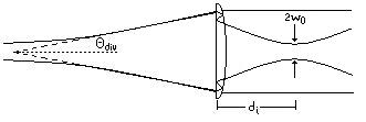
The single lens setup allows for a collimated and focused beam to become collinear due to the internal reflection of the light in the lens[1]. The benefit of this type of setup as an interferometer is that it provides a system that is prone to less error than a classic interferometer. Namely these areas occur in vibrations of the different components, causing the difference in path of the two beams to diminish greatly. This single, or primary, lens is placed in a diverging beam in such a way that the primary exiting beam is collimated. The double reflections inside the primary lens cause a secondary beam, of greatly diminished intensity, to exit with the collimated beam. Since the two beams exit the primary lens at the same point, it is a simply procedure to make them nearly collinear; this allows for nearly perfect viewing of the interference between them.

With the setup described above the incident diverging beam is created by placing an initial lens that tailors the beam to have a specific diameter and divergence at the primary lens. The thing about this initial lens is that it should be placed within the Rayleigh range of the laser. Once outside of the Rayleigh range the laser has a constant divergence, which can then be used as the initial beam for the primary laser. When a lens is placed outside the Rayleigh range it requires a different focal length every distance away from the minimum waist of the laser. This allows for a simpler setup since the only optical element required is a large focal length lens placed at a location such that the beam becomes collimated. The same effect occurs as above and provides the same measurements of the wavefront.

Overview of Gaussian Beam Theory

In this section we will briefly look over the theory on Gaussian beams. The following equation is a solution to the paraxial wave equation[3]:

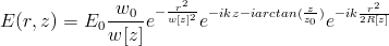
I define w₀ to be the radius of the beam when the curvature of the beam is a plane wave. This means that the waist is at the point where z=0. Everywhere else the radius of the beam is given by:

To analyze what the Gaussian equation does it is simpler to consider three separate parts of the equation: the amplitude factor, the longitudinal phase factor, and the radial phase factor. The amplitude factor is the non-complex portion of the equation. This is the part of the equation squared is the intensity that is measured. The longitudinal phase factor is just a plane wave from the ikz term with a slight correction to push the on-axis part of the wavefront in front or behind of the plane wave. This correction factor is called the Gouy phase term and contributes a total of &pi over all of z. Lastly, the radial phase factor is what changes the wavefront from being planar at the waist to having a minimum curvature at z₀ to becoming a spherical wave outside of the Rayleigh range.

One last important note about this simple Gaussian beams is that they remain Gaussian beams, but with different waist sizes, as they pass through radially-symmetric optical elements.

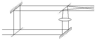
Mach-Zehnder Method

The classical way of viewing the wavefront of a focused Gaussian beam is to setup a Mach-Zehnder interferometer with a lens in one arm (Fig. 1). This allows for there to be a collimated and focused beam to be collinear in the output beam of the interferometer.

To see how this occurs the intensity equation must be derived. Finding the interference pattern is rather simple: just add the two electric fields and multiple by the sums complex conjugate. The top arm creates a collimated beam, which we will assume to be a plane wave, and the bottom arm creates a focused beam. The equations for these two electric fields are then:

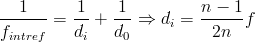
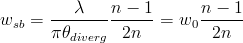
One other important detail is the relative intensity between the focused beam and collimated beam. This comes into account when choosing the focal length lens to put in the interferometer, because the focal length directly determines the waist of the focused beam. The relative intensity is defined by the ratio of the power over the ratio of the areas. I will use a specific equation for calculating the waist:

There are several problems with this setup. One is that both the arms of the interferometer have the same beam diameter before the lens is put into the bottom arm. This means that if a lens is chosen to give a proper sized waist to limit the relative intensity, then the focused beam will be interfering on a non-level section of the reference beam. This does not hamper the visual aspect of the setup, but creates slightly irregular graphs, as will be shown. The two other problems with this setup are purely mechanical. The first is the fact that it is a Mach-Zehnder interferometer, so this causes the setup to be rather difficult to align. The second is that since there are so many components to the interferometer, slight vibrations can cause phase shifts in the focused beam

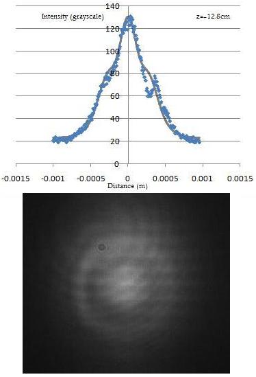
The focal length lens that we used in the interferometer was a 200mm focal length. Due to its distance away from the laser's waist, there was some divergence of the beam, and caused the focused beam to have a waist at 290mm instead of 200m from the lens. I calculated the waist that forms to be 166�m, but this is assuming that the beam comes in with no divergence. In Fig. 2 there is a representative picture from the setup and a slice of the grayscale data.

Ghost-beam Method

Peatross and Pack propose simplified ghost-beam method[1] purely to provide a visualization of the Gouy phase. This setup requires just two lenses, Fig. 3. This setup uses the internal reflections within the primary lens to create a focused ghost-beam within the collimated reference beam.

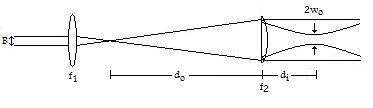
In Fig. 3 we will call the first lens the secondary lens and the second lens the primary lens. The purpose of the primary lens, which is plano-convex (PC), is to collimate the beam and create the ghost-beam. The secondary lens is used to control the divergence of the beam incident upon the primary lens. Also the ratio between the two focal lengths controls the size of the reference beam, since this set up is also the same as a telescope. An important note is that the secondary lens should be placed within the Rayleigh range of the laser to have the beam focus close to its focal length.

The equation for the intensity equation is identical to that for the Mach-Zehnder interferometer. The only difference between these two setups is that the waist of the secondary beam is so much smaller compared to the collimated beam that we can approximate the first electric field to be just the coefficient. This gives an intensity equation of :

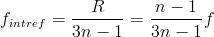
To determine where the ghost-beam will focus and what its size will be requires so additional analysis of the setup. The first step is to determine what the internal-reflection focal length for the internally reflected light will be. To do this it is simplest to use matrix methods to trace the path of the beam as it goes through the plano surface, reflects off the surface with curvature R and then bounces off the plano surface and through the curved surface:

Using the same equation as for the first interferometer, I will need to know the f* of the lens. In this case the f* will be the ratio of di to the beam diameter at the lens, d. Since the secondary lens is located in the lasers Rayleigh range we can say that the beam diameter at the primary lens will be where f1 is the secondary lens and f2 is the primary lens. After some simple algebra we arrive at an expression for the waist to be:

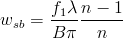
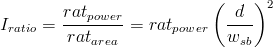
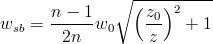
For my setup I choose the primary lens to have a focal length of 1000mm and the secondary lens to have a focal length of 250mm. These lenses should produce a w_sb=33.6�m, a Rayleigh range of 5.6mm, and an I_ratio=1.42. With these numbers I feel that this pair of lenses produces an interference pattern that can be well seen upon the CCD camera. The focus will occur at 16.7cm away from the primary lens. In Fig. 4 there 1pixel slices of the images in Fig. 5.

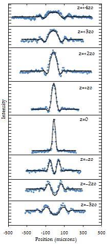
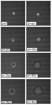
The images at �z0 will have the tightest width of the ring images. This is due to the radius of curvature of the being the smallest. When the focused wavefront intersects with the plane wavefront, the curvature will have the greatest slope at these points, so the fringes will switch from bright to dark faster, resulting in the small fringe widths. Also since the phase has been chosen as + &pi/2 the center spot of the images will remain dark for negative z and bright for positive z.

Single Lens Theory

Since the whole purpose of the ghost-beam method is to visualize the Gouy phase then any means of viewing the intensity patterns in Fig. 5 would be acceptable. I realized that since the presence of the secondary lens was just to control the divergence of the beam incident upon the primary lens it could be removed. Figure 6 is an even simpler method. The beam that is incident on the lens gains its divergence due to the intrinsic properties of the laser.

This method also used a PC lens the equation for the intensity will be the same as for the ghost-beam method. The only difference in the equations occurs when the diameter of the beam starts to be taken into account. This means that the equation for the waist, and therefore the intensity ratio, will be different.

Outside of the Rayleigh range the divergence is almost a constant. When a large focal length lens is placed at a distance so that the reference beam is collimated, then the beam acts as if its waist is located at a focal length away from the lens. With most lasers, especially gas lasers, the divergence satisfies the paraxial approximation. From this I can say that . Now that I know the diameter I can find that 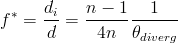. This finally gives an expression for the waist to be:

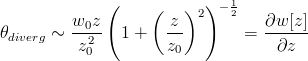
This is also to consider what would happen inside the Rayleigh range. It is possible to approximate the divergence of the beam by using the derivative of the radius equation. This approximation is accurate to the divergence equation to within 0.2% for large z. This gives us a new equation:

Next I need to know where to place the lens. Since the beam is being collimated I consider the waist of the beam to be located a focal length away from the lens. This gives the relation that 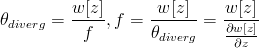. After some algebra an intuitive relation comes out that:

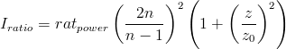
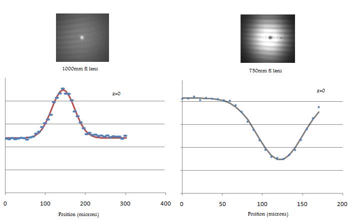
To test this theory I wanted to see if two different lenses could produce the same size waist. In my setup I used a 1000mm lens and a 750mm lens. Figure 7 we took pictures at z=0 and determined the

Summary

I have tested all three of these setups and found that the Mach-Zehnder setup is far less effective in demonstrating the Gouy phase than the other two. Also I have seen that by removing the secondary lens from the ghost-beam method the Gouy phase becomes simpler to visualize. This step of removing the lens requires only the knowledge the divergence of the beam, which is easily determined by beam profile measurements at one or more distances from the laser.

Acknowledgment

This project was supported by the Nation Science Foundation (Grant No. Phys-0851594).

References

[1] J. Peatross and M.V. Pack, Am. J. Phys. 69, 1169-1172 (2001).
[2] P.Nachman, Am. J. Phys. 63, 39-43 (1995).
[3] H. Koglenik and T. Li, Appl. Opt. 5, 1550-1567 (1966)