Studying Rainbow Effects Created
by Sunlight and Laser Beams

Introduction

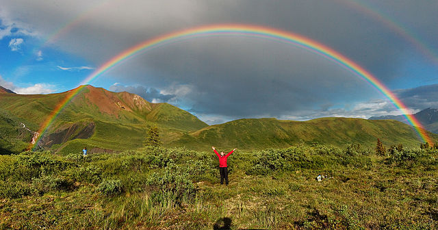
I have been fascinated by rainbows for a long time. I think I was in kindergarten when I first started to be curious about how they are formed. At that time the mechanism seemed like magic to me. Many years later I learned that rainbows have something to do with the refraction of light. My project this fall with Dr. Noé has given me a chance to rainbow effects in great detail and to create some artificial rainbows with a glass sphere.

Rainbow on the Wikipedia

James B. Calvert has discussed the history of rainbow models in great detail. Descartes (1596 — 1650) analyzed the formation of a rainbow in terms of the trajectory of light in one rain drop. Later theories are much more sophisticated and take into account effects such as polarization that can only be observed with optical instruments. In Descartes' model rays of sunlight refract as they enter the drop, partially reflect from the back of the drop and then refract a second time as they leave the drop. The reflected light is concentrated at an angle of about 42 degrees from the direction of the incident light; the exact angle depends on the wavelength (color) of the light, thus creating the beautiful pattern of colors that is observed.

In this project we started by creating a Descarte model in MATHEMATICA. We next created an artificial rainbow with a glass sphere and estimated the rainbow angle with a template. This angle is only about one-half the usual rainbow angle because glass has a higher index of refraction than water. Later, while attempting to measure the index of refraction of the sphere by the Fresnel method with a laser beam we discovered how to create a striking rainbow effect by diffusely reflecting the laser light leaving the sphere. This time we measured the rainbow (concentration) effect more carefully and compared this to a prediction made with MATHEMATICA.

Creating a Descartes Model in MATHEMATICA

We assume that all of the incident rays are parallel to the optical axis and to each other, which is a good approximation. As we can see from the diagram below, the ring of rays that are at the same distance to the optical axis will come out of the sphere in the same angle relative to the optical axis. Descartes proposed that the emergent light is concentrated near a certain angle which is determined by the refractive index. Since sunlight is composed of a range of colors and the refractive index of water for each color is slightly different, light of different colors will form rings of different angular sizes. Those rings are the rainbow we ususlly see in the nature. The concentration angle is around 42 degrees and more than half of the rainbow is normally under the horizontal line because the sun above the horizon. Therefore, rainbow often appears as a bow, not as a full circle. From an airplane or mountain top one could possibly see the complete circular rainbow.

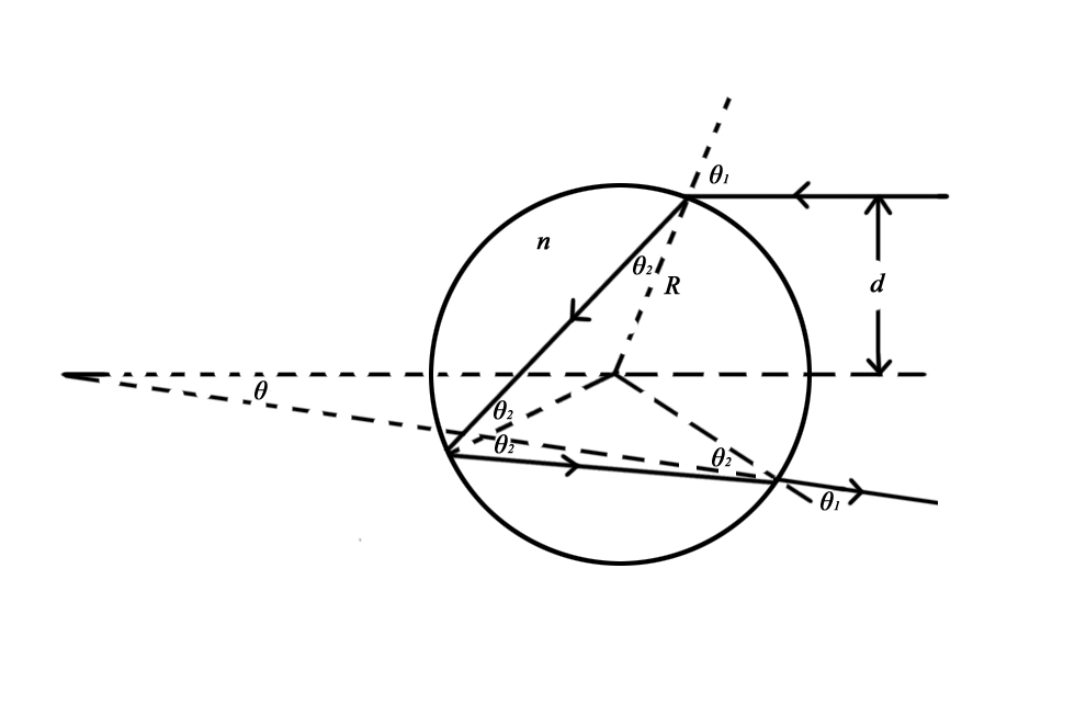
Schematic Diagram of Descartes' Model

With simple geometry, we can use this model to explain the rainbow effect quantitatively and even make a rainbow on a computer. The angle between the emergent light and the optical axis (deviation angle) can be expressed in terms of the refractive index of the raindrop n and the ratio of the distance between the incident beam and the radius of this raindrop x:

The range of the variable x is between 0 and 1. With n=1.33 a plot of the deviation angle versus the ratio x can be drawn with this equation:

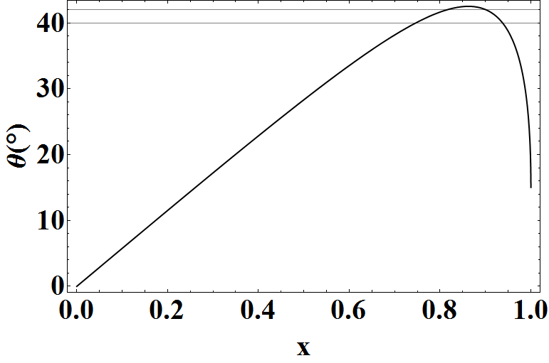
θ-x Plot

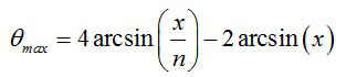
As demonstrated in this figure, the deviation angle has a maximum value when we change x from 0 to 1. We can obtain this maximum angle by differentiating the equation above:

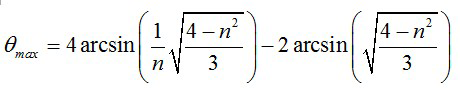
This maximum deviation angle is about 42 degrees, and this value depends only on the refractive index n. However, the concentration effect is not explicitly shown in this figure. We can use the following method to show the concentration effect. It is reasonable to assume that the intensity of incident beam is homogeneous on the cross section. Since the deviation angle is determined by the ratio x, we can first consider a ring with the width of Rdx. All the rays that goes through the ring with the width of Rdx will come out of the sphere in a certain range of deviation angle dθ. The smaller the dθ is or the larger dx is, the more concentrated the emergent light will be. Therefore, we can define the concentration density as dx/dθ, which indicates the degree of concentration in a certain angle. We can plot the concentration density of red, green and blue light versus the deviation angle with n = 1.331, 1.3334 and 1.3362 for those colors.

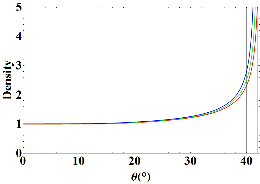
Concentration Density Curves for red, green and blue light

The concentration density for each color increases rapidly in the range of 40-42 degrees as we expect, which means the concentration effect happens around the maximum deviation angle. Moreover, the concentration angle is different for each color. The concentration angle of blue light is the smallest and that of red light is the largest. This is why different layers of color can be seen in the rainbow. In the region where θ is smaller than 40°, the concentration densities of three colors nearly have the same value. They overlap each other to produce the white light. We can numerically simulate the rainbow with three colors in MATHEMATICA as shown below:

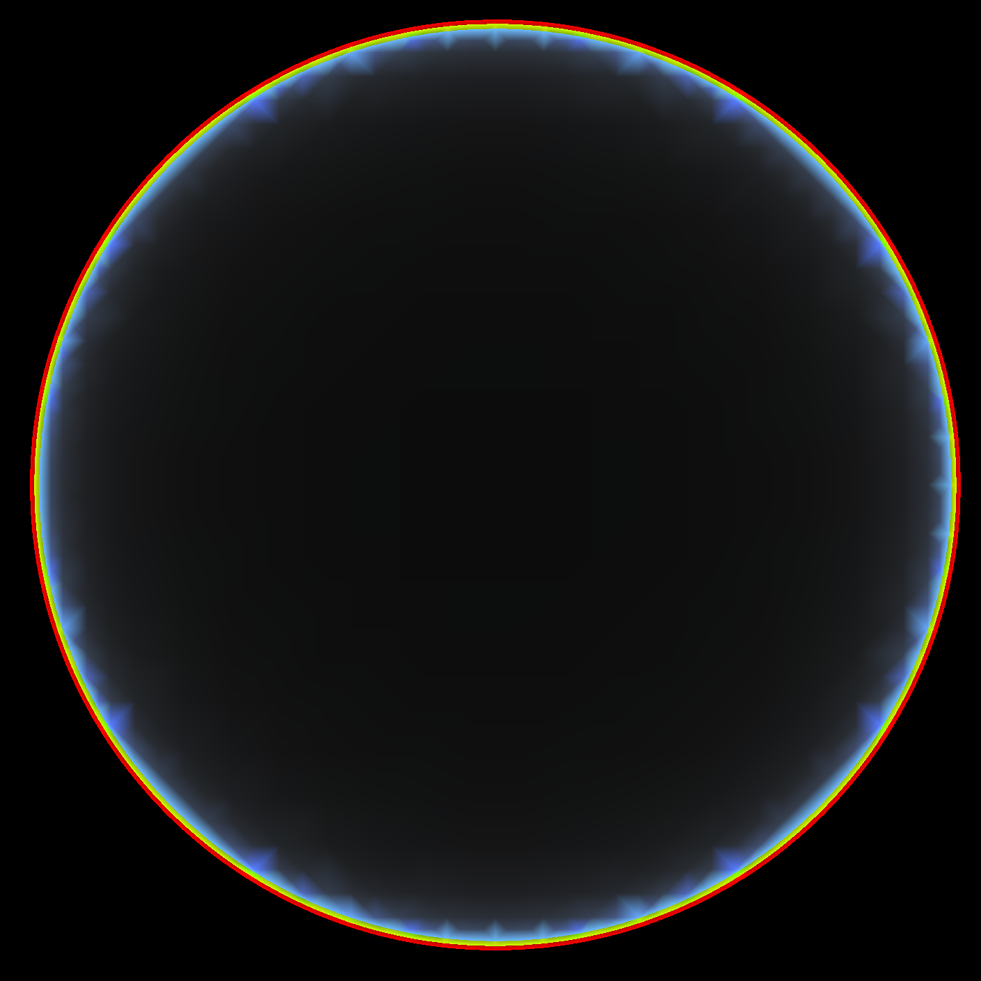
Simulation of Rainbow on Computer

Creating an Artificial Rainbow with a Glass Sphere

We also created an artificial rainbow with a glass sphere. We measured its diameter and weight to be 11.00 and 1729 grams, respectively, so its density is 2.50. This is consistent with ordinary glass.

We put the sphere in direct sunlight and used a template with a hole on it (slightly larger than the sphere) as a screen. We moved the template slowly until we could observe a distinct uniform rainbow. Pictures from this demonstration can be seen in the Pictures section. We used the equally spaced circles on the template to measure the diameter of the outermost edge of the rainbow, which should correspond to the concentration angle of red light, at a few different distances from the sphere. The concentration angle can be deduced with the data.

Let D be the distance between the center of the sphere of radius R and the screen, and let y = D/R. Then the radius of the ring corresponding to the deviation angle θ can be expressed in y, θ and the dimensionless impact parameter x as follows:

Our experimental result for the concentration angle of red light was about 20°, which is only about half of 42°. The much smaller concentration angle compared to that in a natural rainbow is because the typical refractive index of glass (1.5) is larger than that of water (1.33). For example, an index of n=1.51 corresponds to a concentration angle of 21.9°. A spherical flask of water could be used to make a more realistic demonstration. Our angular uncertainty was rather large (at least ±1°), largely because we couldn't hold the template screen steady enough. The experiment could be improved by mounting the screen on an adjustable frame.

Creating and Modeling a "Laser Rainbow"

We studied this laser rainbow effect in detail. We used Witeout(TM)instead of paper later on. This concentration effect is created by light reflected from the back of the sphere. When we put a piece of paper on the back of sphere, light beam was reflected back and then concentrate in some certain angle. The following schematic diagram shows this effect and there are pictures in the Pictures section

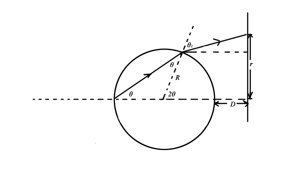
Schematic Diagram of Laser Rainbow

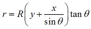
We can deduce the radius of the ring with respect to θ, D and R shown in the diagram.

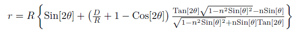
r-θ curve

As we can see in the figure, there is a maximum value of r. This is similar to the θ-r curve of the real rainbow. And this maximum radius is the concentration radius. Since the concentration angle of the rainbow is determined by the refractive index only, we decided to use the maximum radius of laser rainbow to deduce the refractive index of the sphere.

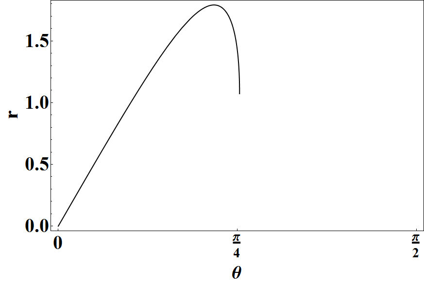
We carried out some careful measurements of the diameter of the outer edge of the ring at different distances between the screen and the sphere. At each distance we marked the two opposite outer edges of the ring on a foam-board screen with a small hole in it. We were careful to set the screen perpendicular to the table top. Before making the measurements, we carefully adjusted the setup to make sure that the laser beam went through the center of the sphere. We tilted the laser to make the laser beam parallel to the table and adjusted the height of the sphere until the spots of reflected light from its front and back surfaces overlapped each other on the screen. We observed unexpected interference fringes when the two spots were overlapped. The data we obtained appear to be highly linear, which means that the angle of the outer edge of the ring and the table is a constant. If we use this obtained angle (which was about 11 degrees) as the maximum angle, we can deduce the refractive index of the sphere, with the result n = 1.51. The sphere is actually made of glass not plastic! This graph shows our data with a straight line fit.

However, we later realized that this is not the whole story. Light from the maximum angle does not necessarily form the outer edge of the ring. The concentration we saw with our eyes is due to the limit of maximum radius, but not the limit of maximum angle in this system. It turns out that the condition of the maximum radius is closely related to the position of the screen. Our explanation of the "laser rainbow" may not be complete, since we only took the maximum angle into account. The peak of the radius with respect to the reflective angle actually shifted when we moved the screen back and forth, which means the angle of the outer-most light is not the maximum angle.

In order to get a better understanding of this effect, we used the formula above to draw the following schematic diagrams.

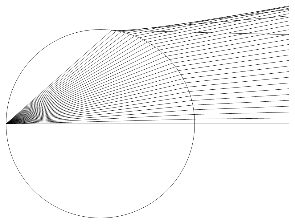
Ray-tracing diagram showing near-field regime

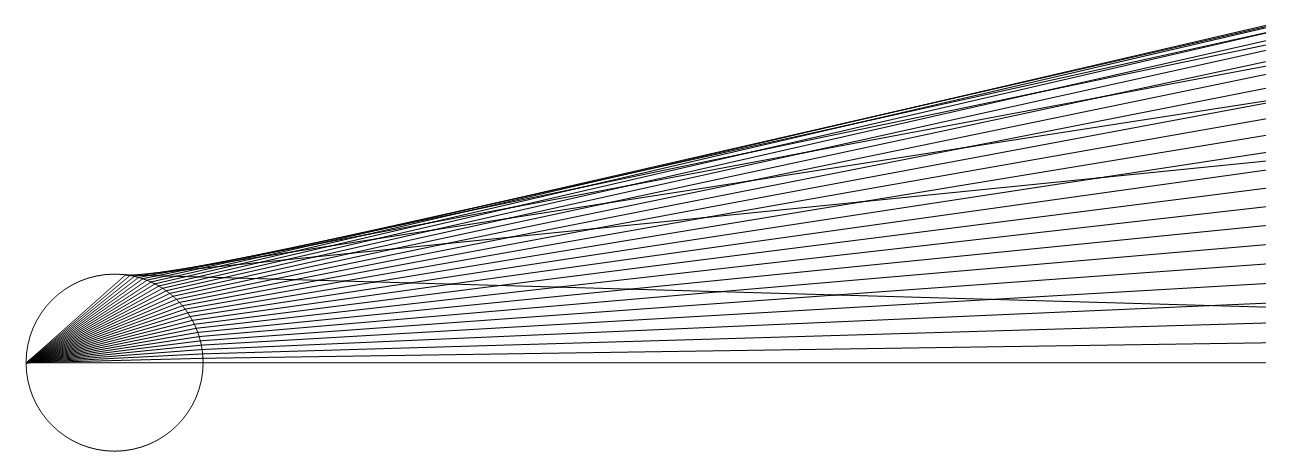
Ray-trace diagram showing far-field regime

As we can see in the diagram, at different distances the outermost edge of the ring is formed by rays which correspond to different θs. The outermost edge is actually an envelope of rays. Close to the sphere the relationship between the maximum radius r and the distance D is not linear. However, far from the sphere the envelope of rays approaches its asymptote, which is a straight line. That is why we can fit our data with a straight line and still achieve very good result.

We can do the analysis in a more precise way by non-linear fitting. By setting the derivative of r over θ equal to 0, we are able to obtain the condition when r reaches the maximum value. We have known that the index is around 1.5. Therefore, we first tried to plug n = 1.49, 1.50 and 1.51 into the condition we have obtained. The distance D in the measurement ranges from 2R to 13 R. We can solve for the angle θ at every D in that range with the step 0.01R. By using interpolating function, the numerical relation between the maximum value of r and D can be obtained. Those three curves are shown below:

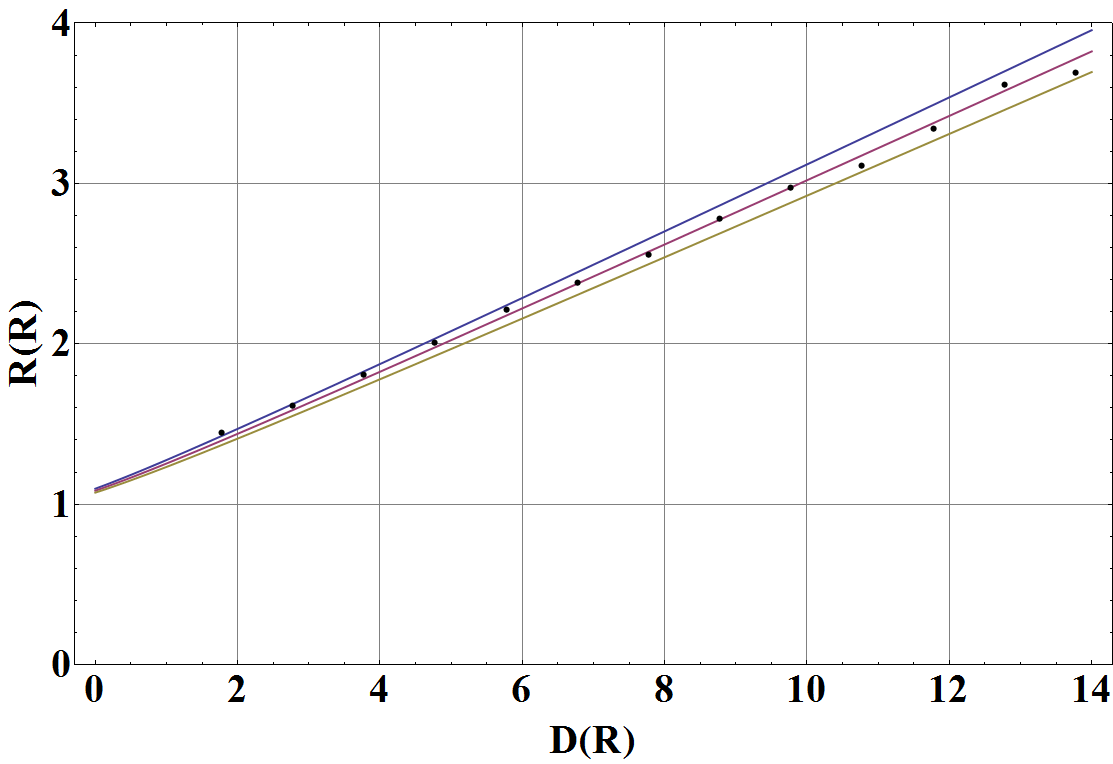
r-D Curves with n = 1.49, 1.50 and 1.51

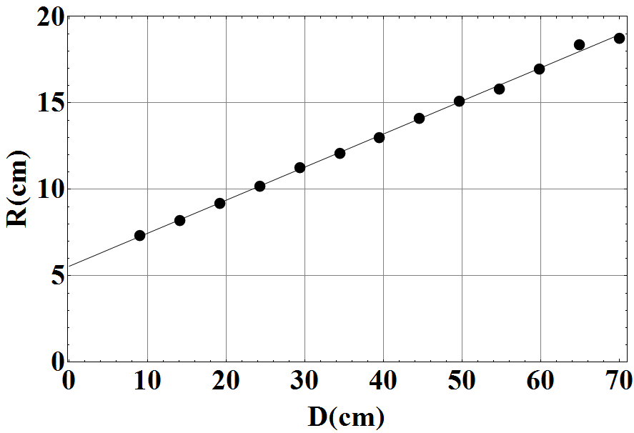
Our data lie about mid-way between the curves with n=1.49 and n=1.51. We used the least square method to find that the best agreement between data and calculation is for n=1.501, as shown below. In this figure the red and blue dashed lines are tangent to the calculated curve at the two sides of the graph. These lines make it clear that the calculated relationship is not precisely linear.

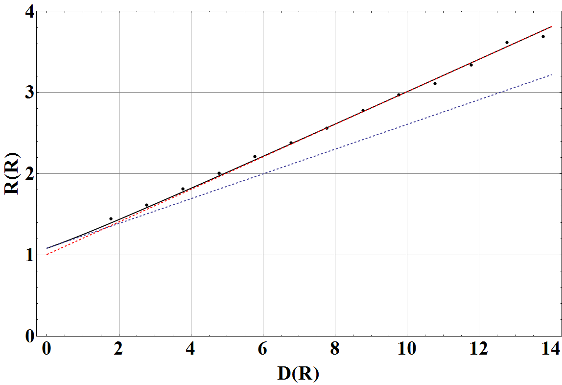
Best fit with n = 1.501

Discussion

In an actual rainbow the incident sunlight covers many raindrops and what we observe is a concentration effect in the angle of the reflected light seen by an observer looking towards the raindrops. In our two demonstrations there was only a single sphere and what we observed is a concentration of light at a particular radius on a screen. Of course the radius of the ring on the screen is related to some angle, but the vertex of this angle lies behind the sphere not on its front surface. Therefore a careful analysis is needed to predict the results of our two experiments. In other words, for a given position of the screen, rays that fall at the maximum radius, do not necessarily correspond to the maximum deviation angle. However, if the distance to the screen is relatively large the maximum radius will be nearly proportional to the maximum deviation angle. Our two demonstrations differ in that in one case the incident sunlight covers the whole sphere while in the other case the laser beam diameter is much smaller than the sphere. (The scattered laser beam is even smaller than the incident beam due to the focusing effect of the front surface of the sphere.) Both sunlight and the laser beam have some angular divergence, but in both cases this small divergence, 10 mrad or less, will cause just a slight smearing of the edges of the ring of light.

In the analysis of both demonstrations, the ring radius and the deviation angle both have maximum values. In the solar rainbow case, we have used the concentration density to indicate the degree of concentration of the emergent light in every angle. This quantity is in fact comprised of two parts. The graph of x-θ (This curve can be obtained from &theta-x curve) has one part below the turning point, and one part above the turning point.

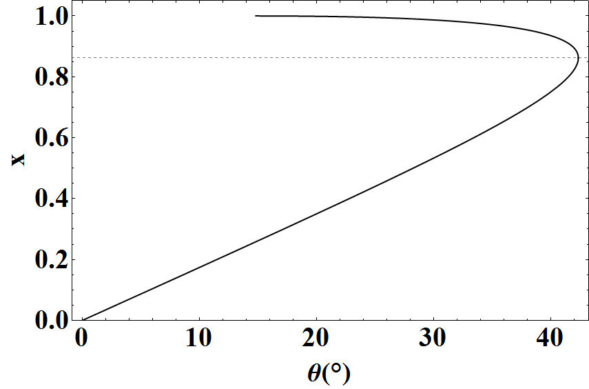
x-θ Plot

When we calculate the concentration, we add the absolute value of both concentration densities calculated from those parts up. In the turning points, both of these two pieces reach their maximum values, which approach infinity. Therefore, we can also define the concentration density which indicates the degree of concentration in each radius as well. With the same method, we can reach the conclusion that there is a concentration around the maximum radius. Also, we are able to do this to the deviation angle in the laser rainbow, which has a maximum value as well. However, this time, the density does not mean anything in our measurement since what we observed on the screen is not directly determined by the deviation angle. Therefore, the concentration in rainbow effect has a similarity that one observable quantity has a maximum value and the concentration effect happens around there. It is important that this quantity can be directly observed. If we use different ways to observe the rainbow effect, we may observe different concentration effect.

Finally, we have seen that in the laser rainbow demonstration the curves of maxiumum ring radius versus screen distance that we generated numerically are quite sensitive to the refractive index of the sphere. Therefore our method can be used to easily determine an accurate refractive index for a sufficiently large sphere.

References for Further Study

Many books and articles have been written about rainbows and rainbow effects. One good source - especially concerning the long history of rainbow studies - is the American Journal of Physics (AJP).

Wikipedia article on rainbows

Optics Picture of the Day (OPOD). Has many "galleries" related to natural rainbows and other atmospheric optics effects. This gallery shows a laboratory demonstration of the first six orders of rainbows.

Website of Dr. James B. Calvert (http://mysite.du.edu/~jcalvert/). Very thorough discussion of the theory of rainbows.

Marcel Minnaert, The Nature of Light and Colour in the Open Air. Dover books reprint, 1954.

Giovanni Casini and Antonio Covello, "The rainbow in the drop," AJP 80, 1027 (2012).

David Skid Amundsen et al, "The rainbow as a student project involving numerical calculations," AJP 77, 795 (2009).

Harold A. Daw, "A 360° rainbow demonstration," AJP 58, 593 (1990). Uses a partially-silvered sphere to enhance the rainbow intensity.

Frank S. Crawford, "Rainbow dust," AJP 56, 1006 (1988). Rainbow effects that can be observed with tiny glass beads, commonly used on road surfaces.

Jearl D. Walker, "Multiple rainbows from single drops of water and other liquids," AJP 44, 421 (1976). Very thorough geometrical analysis of rainbow effects of various orders.

Bruce S. Eastwood, "Robert Grosseteste on Refraction Phenomena," AJP 38, 196 (1970).

Carl B. Boyer, "William Gilbert on the Rainbow," AJP 20, 416 (1952).

Carl B. Boyer, "Kepler's Explanation of the Rainbow," AJP 18, 360 (1950).