Research Journal
Spring 2014
Wednesday April 30 2014
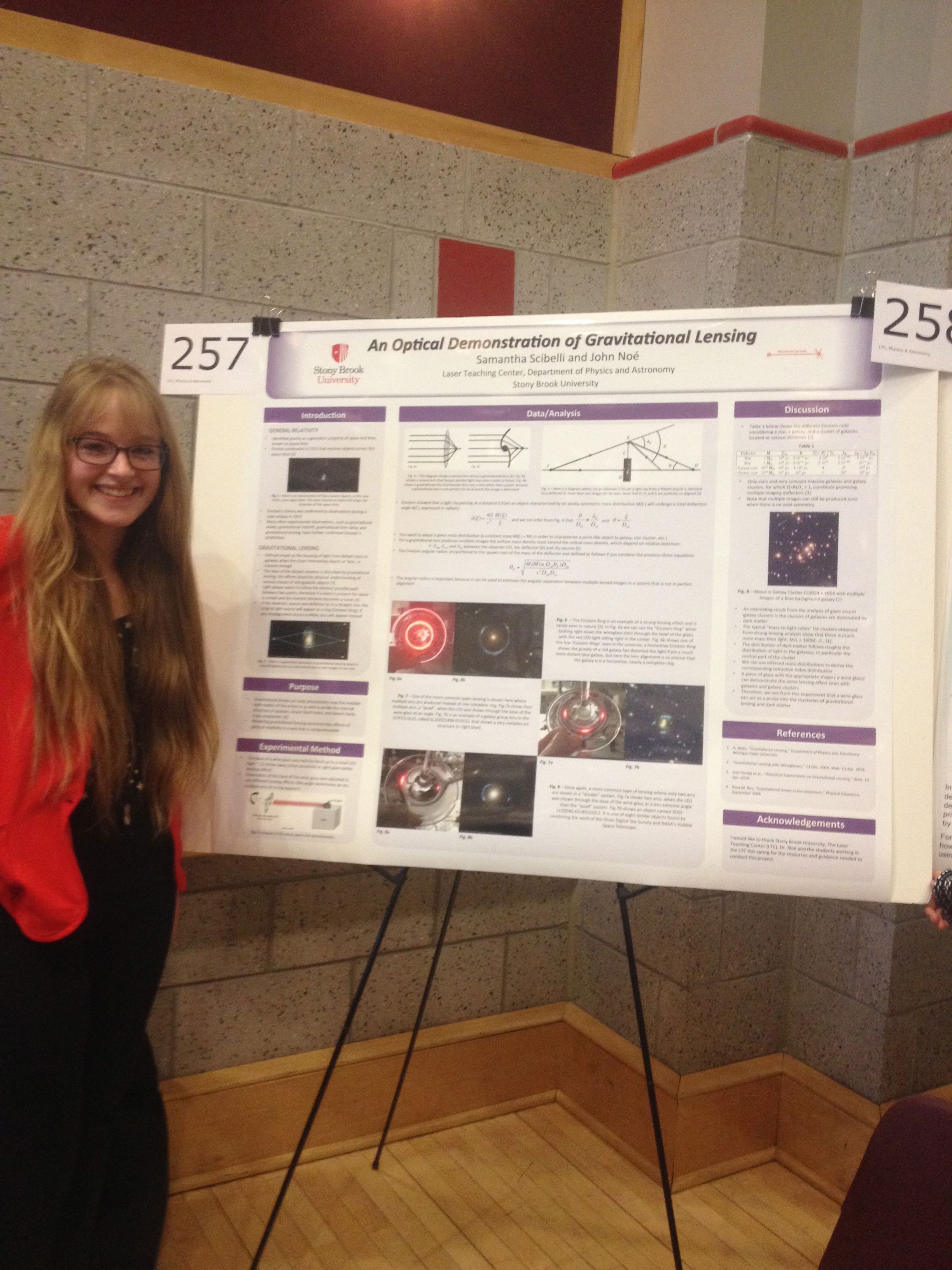
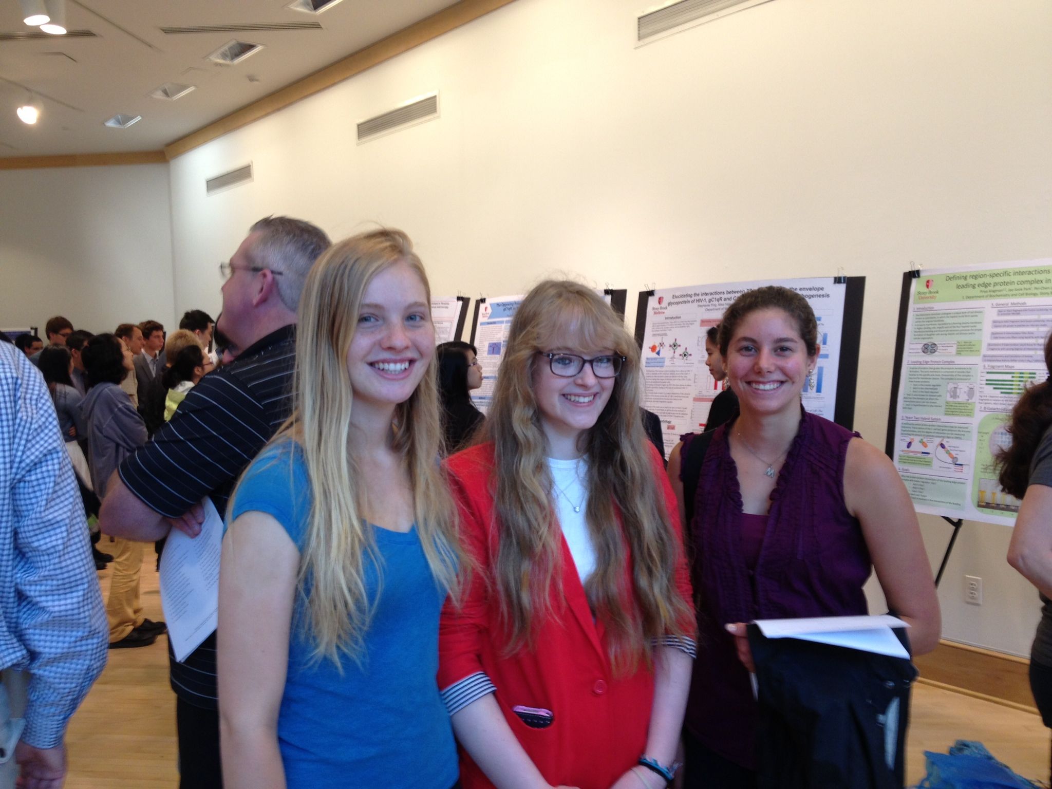
Today the LTC group presented at URECA! I had a lot of fun presenting my poster and showing other students the various optics demonstrations at our table. The students were especially interested in the pig ‘mirage’ toy and the diffraction grating glasses. I also had the opportunity to walk around and see the other research posters. I listened to my peers talk about a wide variety of topics such as crystal structures, Gaussian beams, and gas clouds around stars. It was great seeing so many undergraduates presenting research! Overall, I had an amazing time!
Friday April 18 2014
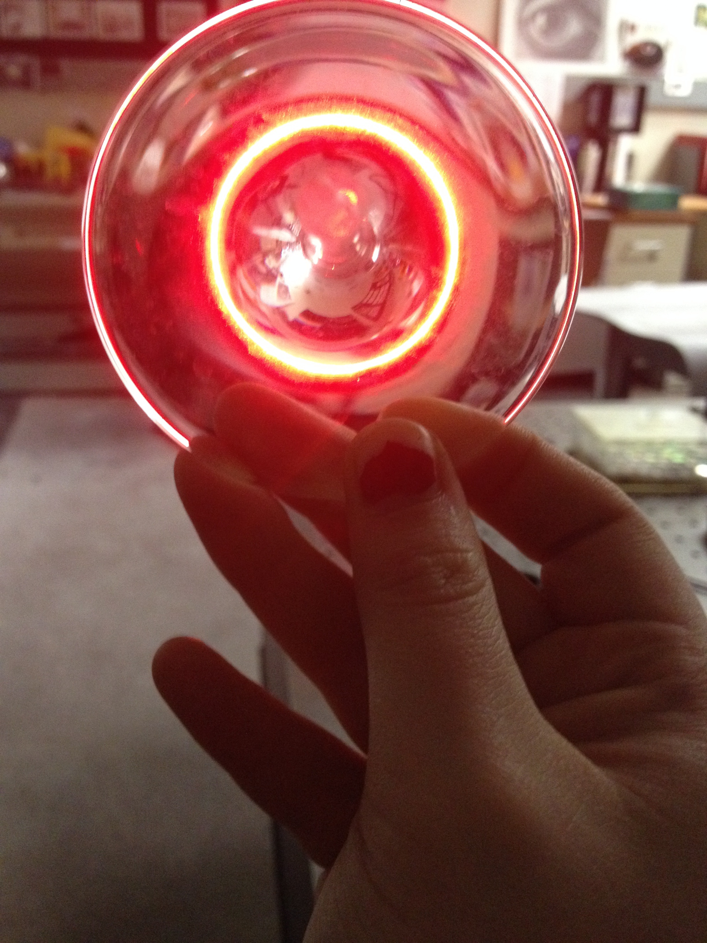
Today in the lab I took some nice pictures of the lensing effects with the wine glass base (see picture below). I experimented with placing the wine glass base at various distances from the LED light. I found that I could more easily see ring and arc structures if I was about twelve inches away from the light. So, I took a series of pictures of different arcs that appears when I titled the wine glass base at various angles from that distance. I also noticed that using the red LED light was visually more appealing than the green, blue or white light. After taking a few dozen pictures, I helped Natalie set up her fractal display where she used silver ornaments and the same LED lights I had been using. The fractal patterns we saw were really neat! Today I also started working on my poster for URECA, gathering pictures and organizing the layout. I am really excited for URECA where I will be able talk about my knowledge of gravitational lensing with other undergraduate students!
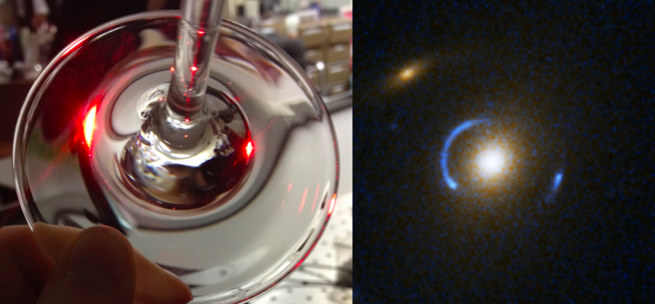
Monday April 14 2014 Over the weekend I had the opportunity to read more on gravitational lensing and the mathematics behind it; I went over calculations with the lens equation and calculations of the Einstein radius. I also watched a talk by Marusa Bradac, who gave a talk at Stony Brook titled Shedding Light on Dark Matter: Seeing the Invisible with Gravitational Lensing. She explained how multiple images and distortions made by gravitational lensing could tell astronomers about mass distribution. She even mentioned using a wine glass to show this effect! Also, in lab today Libby, Natalie and I were able to finish our abstracts for URECA.
Friday April 11 2014
During todays group meeting I was able to work on my abstract. I spent my time gathering information on the history of gravitational lensing and it’s implications in both physics and astronomy. I read up on Einstein’s theory of general relativity. Einstein saw gravity as a geometric property of space and time, known as space-time. He realized that massive objects could distort this space-time. Gravitational lensing is one of the several observable effects of this theory, others being gravitational waves, gravitational redshift, and gravitational time delay. Also, I was able to take some preliminary pictures of the gravitational lensing effect seen with a wine glass! Below is an image of a classic ‘Einstein ring’ that occurs due to extreme strong lensing effects. This is rarely seen in nature.
Friday April 4 2014
Today in lab Libby, Natalie and I settled on projects! After discussing possible project ideas we decided to settle on projects that were simple yet deep enough to create a project and still finish in a relatively short amount of time. I have decided to model gravitational lensing, creating both physical models and computer simulations. Gravitational lensing can be seen by look at a point source of light with a wine glass. In the days to come I will be busy researching this topic and starting my abstract for URECA.

Thursday April 3 2014
I’ve been reading more on diffraction with feathers. I found a lab procedure online that spelled out how one could find the size of feather structure elements from measuring the periods of the diffraction picture and the distance between the feather and the screen that the picture appears on. They use the equation d = λD/L; where L is the distance between the feather and the screen, D is the period of the diffraction pattern, λ is the wavelength of the laser, and d is the period of the feather structure responsible for the pattern. They did this experiment with a rooster, hen, duck and goose feather.
The results show that bird feather has a structure with two scales and two directions. The smaller one has the period of several microns, and larger one is of the order of hundred of microns. These features that cause the diffraction patterns can really be seen if you look through a microscope lens.
Friday March 28 2014
Today Dr. Noé, Rachel, Libby and I went to lunch at the Simons center to meet with a prospect WISE student and her family. After lunch we went back to the lab and continued brainstorming project ideas. After brainstorming, I created an ideas page, which list names and links of possible project topics.
Wednesday March 26 2014
Today I read an article about using feathers to create diffraction patterns. A 17th century Scottish mathematician, astronomer and physicist James Gregory used a bird feather to split a beam of sunlight into different colors. He saw this effect just a year before Newton made the same famous observation. But unlike Gregory's plain bird feather, which produced multiple spectra, Newton used a glass prism to produce a single spectrum. In turns out that the feather grating did not become the favorite method. I think it would be interesting to see the diffraction patterns that various feathers do make. In addition, the article mentioned using a feather in a device called "X-ray Specs" that gives the illusion of seeing inside an object. This sounds like an interesting mini-project to look into. Perhaps after I read a few scholarly journal articles on this topic I can craft a project out of this idea.

Friday March 14 2014
Today in the group meeting Dr. Noé taught Natalie and Libby the basics of running a webpage and writing their own journals. Also, Dr. Noé gave me an interesting article to read titled, Angular Momentum Transport in Astrophysics and in the Lab. In this article the goal of the physicists experiment is to better understand astrophysical accretion disks. Accretion disks are important to the process of star formation and can teach us a lot about how the stars in general form. The flows can’t be directly observed so the physicists are creating them in the lab! They do this by using Laser Doppler velocimetry, using the Doppler shift in a laser beam to measure the velocity in transparent or semi-transparent fluid flows, or the linear or vibratory motion of opaque, reflecting, surfaces. Laboratory experiments uses two concentric cylinders – an inner cylinder that rotates at angular velocity Ω1 and an outer one rotating at Ω2. Using either water or liquid metal as a medium and choosing Ω1 < Ω2 and R12Ω1 < R22 Ω2, physicists can set up the conditions relevant for studying the rotational dynamics of accretion disks! It’s amazing that the Doppler shift can be used to model so many different processes in our universe!
Tuesday March 11 2014
Today I read some articles on rotational/angular Doppler shift. I began by reading a short article by Miles Padgett that Dr. Noe had recommended. It discussed how light with an angular momentum will undergo a frequency shift when it bounces of a rotating object. This effect was demonstrated in the 1970s when a circularly polarized light beam was rotated about its propagation axis. It had a rotational velocity, Ω, and its frequency was shifted in accordance with Δω=σΩ, where σ = ±1 for right- and left-handed circularly polarized light. Padgett explained the frequency shift very well by stating that you could “think about a second hand on a stopwatch, which is analogous to the electric field vector in a circularly polarized light beam. If the stopwatch is placed face up on the center of a turntable, the revolution of the turntable cause an observer in the rest frame to see the second hand rotating at a different speed.” In his experiments he used a rough surface to scatter light off to test the effects. He used a forked grating to measure the intensity modulation resulting from the Doppler shift of two beams with opposite orbital angular momentum values scattered from a spinning disk. Him and his colleagues found that the rotational Doppler effect might allow for sensitive measurements of ration, even when the conventional Doppler shift is absent.
I read another article from physicsworld.com. Martin Lavery and his colleagues at the University of Glasgow, together with researchers at the University of Strathclyde, did an experiment where they stuck a piece of aluminum foil to a wheel that was spun by a motor taken from a remote-controlled car. Two superposed light beams of the same frequency and intensity but with equal and opposite angular momenta illuminated the back of the foil. They found that when the light hit the rotation surface, the two beams are affected slightly differently. This was because the angular momenta relative to the spinning surface are different. The frequency of the scattered beam with orbital angular momentum in the same direction as the surface is raised slightly (blue-shifted), while the frequency of the beam with angular momentum in the opposite direction is lowered (red-shifted) by the same amount! Their group published a paper on their work so I plan to reading about their results more thoroughly.

Friday March 7 2014
Last Friday Dr. Noe showed demonstrated Doppler shifts that occur when using a Michelson interferometer. I was curious about this device and decided to research it more in depth. I previously read about it in my astronomy textbook this semester when we were discussing telescopes. The set up is pretty simple; I even found this great YouTube video that describes in depth how you would measure the wavelength of the light. The interferometer is composed of a laser, an adjustable mirror, a movable mirror and a beam splitter (in telescopes there is also a detector). Basically by seeing how the intensity changes as the mirrors are moved we see different patterns of the light constructively and destructively interfering. Each time the pattern returns to an identical position, the mirror has moved half a wavelength. Therefore by counting the number of cycles we can measure the wavelength.
Tuesday March 4 2014
Today Natalie and I attended a talk by the Nobel laureate, Frank Wilczek, at the Simons Center. The talk focused on how we perceive light and, therefore, how we receive reality. I have always been fascinated by light and this talk reminded me of the many questions I use to ask myself when I first learned about the electromagnetic spectrum. Such as, what if we could detect IR or UV light? What would we see? Would they be seen as a completely new colors? It seems unfathomable to me. Would we think about our world any different? I thought about something I read for my anthropology class this semester, an anthropologist had said that humans are the only animals that do not live in the real world. In that context the anthropologist was referring to how humans live in a reality formed by the culture in which they live. However, after thinking about this and listening to Wilczek talk, I think that statement could also be true because of how we actually see the world. We see the world differently from many animals and who is to say whose reality is the ‘right’ one? How do we know what we are seeing through our eyes is really an accurate representation? What else is out there that we can’t see? We know there has to be something, don’t we? We already know that the universe is only four percent of the stuff we can actually see! The rest is this strange dark matter and dark energy. That’s mind-blowing! Hopefully someday my questions will be answered, but for now I will keep asking them.
Friday February 28 2014
Today in the lab I gave a brief talk on the Doppler effect. I began by using an analogy of a bug sitting on the surface of a pond. By moving its arms the bug creates concentric circles, where one side of the circles we label a point A and the other side we label a point B. If the bug is stationary then the frequency of these water waves is the same regardless of whether or not it’s being observed from A or B. However, if the bug starts moving towards B, the observed frequency will change. Point A will observe a lower frequency and point B will observe a higher frequency. It’s important to note that the actual frequency isn’t changing. This is a basic example of the Doppler effect. The Doppler effect works with any type of wave, whether it is water waves, sound waves, or light waves. A common example of the Doppler effect is a police car siren. When the police car is moving towards you, you hear the pitch of the siren increasing and then decreasing as the car drives away from you.
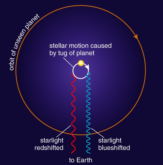
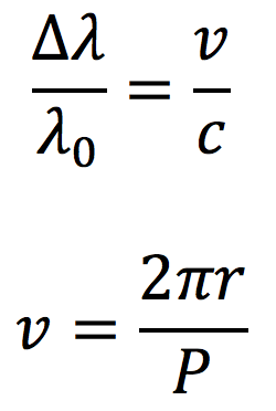
The Doppler effect has also been a crucial part of astronomical research. Astronomers use the Doppler effect to derive information about stars and galaxies. For example, the Doppler shift allows astronomers to detect the slight motion of a star caused by an orbiting planet. How do they do this? By measuring the spectrum of a star as it wobbles (due to the tug of an orbiting planet) we can see the starlight being redshifted as it moves away from us and blueshifted as it comes closer to us. The image below demonstrates this effect. The greater the shift, the greater the relative speed between the source and the observer. Once we know the speed from the first equation shown below, we can calculate the star’s orbital period from the second equation shown below.
Friday February 21 2014
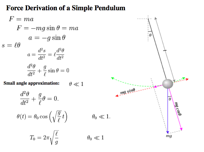
Back in the LTC we continued discussing the idea of the simple pendulum. I spent time going through the calculations on the white board and did some independent research of my own to see how the formula for a period of a simple pendulum can be derived. It’s clearly much simpler when the small angle approximation is used. The derivation is shown below:
Earlier that day I had read an interesting story about Galileo on a hyper physics about the young Galileo that connected to simple pendulums. He made a breakthrough discovery while he sat bored during a church service in Pisa. The chandelier overhead swung gently back and forth, but it seemed to move more quickly when it was swinging widely and more slowly when it wasn’t moving as far. He was curious about this so he measured how much time it took each swing, using the beating of his own pulse. He found that the number of heartbeats between the swings of the chandelier was roughly the same, regardless of whether the swings were wide or narrow. The size of the oscillations – how far the pendulum swung back and forth – didn’t affect the frequency of those oscillations.
Thursday February 20 2014
It feels great to be back in the LTC for the spring semester! Today two other physics majors (Natalie and Libby) and I met with Dr. Noé for an introductory meeting. We discussed possible topics that could be manifested into projects. Libby was interested in fog rainbows and atmospheric optics in general. Both Natalie and I are interested in astronomy and want to incorporate it into our projects. I have been looking into various interferometers in telescopes. Specifically the Michelson interferometer, where incoming radiation is split into two beams, which are reflected off mirrors so that they come back to the same location and interfere with each other.
During our meeting Dr. Noé guided us through various exercises in order to convey the idea that we should be focusing on one simple topic to understand completely. It really is amazing how much we think we know about something, only to then realize how little we really know when we start getting asked questions. For example, today we spent a long time discussing the sin(x) and cos(x) functions. Libby drew various configurations of the function. Questions were asked such as, what’s a radian? Even though all three of us knew the unit and in fact use it every day in class, we never really thought about what that unit actually means. What we realized is one radian is the length of a corresponding arc of a unit circle, where one radian is equal to about 57 degrees. We also discussed the small angle approximation and it’s implications. I will be researching this idea more in depth and hopefully I will be able to fully understand the idea of the simple pendulum by the end of tomorrow's meeting.
Summer 2013
Friday August 9 2013
Thursday August 8 2013
Today marked the official end of my summer research in the LTC. But, I won’t be gone for long ☺. I plan to continue my research once I begin classes in the fall. My time here has been an amazing learning experience. Not only did I benefit from creating my own project, but I have also been able to learn a lot about the other projects in the LTC, which has been great!
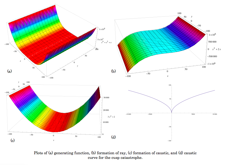
Today I began to familiarize myself more with the equations that create the ultimate shapes, or caustic curves, of the catastrophes. When I continue my research I will pick up on studying the functions of the elementary catastrophes so I can compare them to my observations. Today I also made the remaining plots of the family of functions for the umbilic catastrophes (yay!). But, there is still a lot of work to be done.
So, the geometry of fold and cusp are relatively easy to visualize because the graphs can be embedded in low-dimensional spaces. Higher dimensional catastrophes are more difficult to visualize. So, when I attempt to create diagrams for the higher dimensional catastrophes I could use bifurcation sets that are simpler to visualize since they are embedded to a control parameter space.
Wednesday August 7 2013
The high school students and I had our final summer project presentations at pizza lunch. It was a nice way to wrap up the summer by seeing how far everyone has come in his or her project. Each project is truly amazing and unique, tailored to everyone’s interests. The fact that we each get to pick a project we can be passionate about really makes the LTC a special place. The amount of work that each of us has done this summer is incredible! But I’m sure most of us don’t think of it as work ☺.
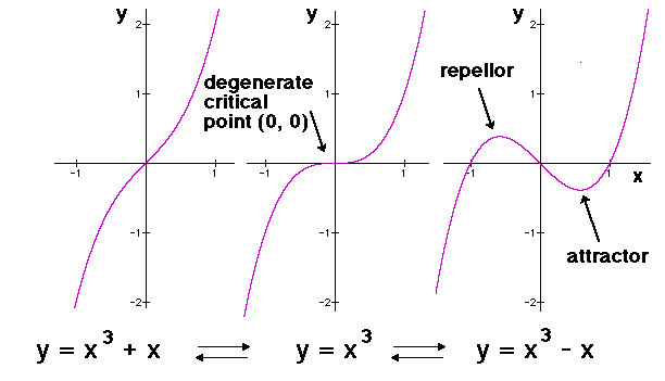
Today I also delved further into catastrophe theory as I continued reading the paper by Gilmore, exploring the changes that can be seen as control parameters change. The generating equation for each catastrophe can form a family of functions based on quantitative changes in the control parameters. I created in Mathematica family of functions for the first four catastrophes; the fold (A2), the cusp (A3), the swallowtail (A4), and the butterfly (A5). These are known as cuspoids and depend on only one state variable (so I can easily plot them in two dimensions but it is possible to plot them in three dimensions and I have done so as well). The last three catastrophes, the elliptic (D4), hyperbolic (D4) and parabolic umbilic (D5), depend on two state variables. The subscript denotes the number of critical points generated, i.e. for a fold (A2) there are two critical points. When critical points of higher order catastrophes annihilate they become a shape of lower order.
I find this relatable to the evolution I am seeing from the evaporating water droplets. When the elliptic umbilic and fold merge into a parabolic singularity, they essentially annihilate at the critical points. Hence, the reversal process can be explained by the idea that once this higher singularity is met a “catastrophe” happens and the lower order catastrophe shapes re-appear.
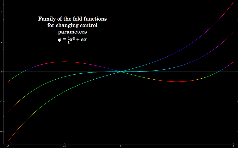
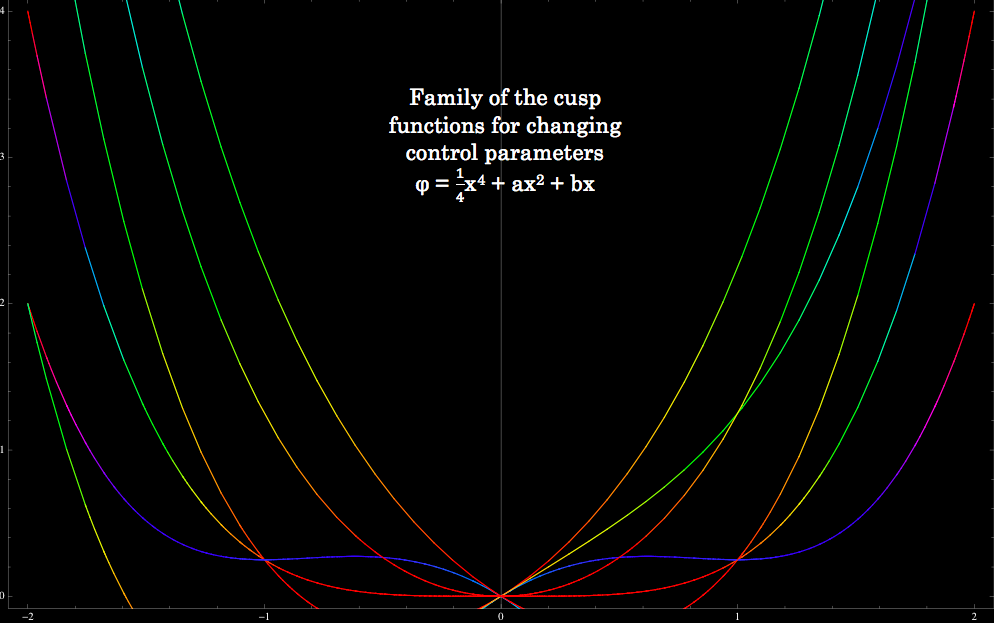
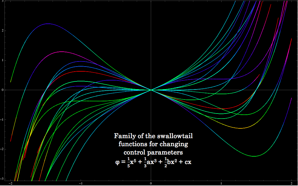
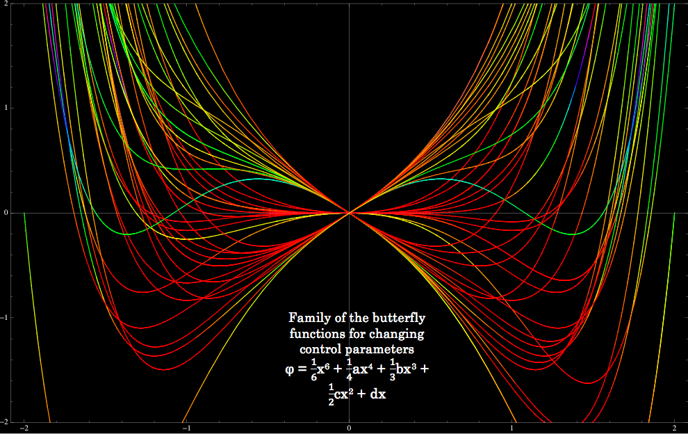
Above you can see the family of functions for the first four catastrophes. A clear relationship can be seen among them. Notice how there are more functions in the higher order catastrophes because, unlike the fold catastrophe that only has the control parameter a, they have more than one control parameter. In the cusp the control parameters a and b are varied. In the swallowtail the control parameters a, b and c are varied. In the butterfly the control parameters a, b, c and d are varied. These plots are pretty awesome looking! The plot of the family of functions for butterfly catastrophe is pretty fitting ☺. I have also plotted the formation of the ray (critical point) and the formation of the catastrophe (the degenerate). My next step is to try and create the shapes of the umbilics, which as I mentioned previously depend on two state parameters.
Tuesday August 6 2013
This morning Melia helped me make my poster for Friday perfect. She also sent me a wonderful link that brought catastrophe theory down to a level that could be easily understood. In this New York Times article, the author explained how the economic crisis and sleep loss are because of this mathematical natural rule. Basically it all comes back to this idea of an equilibrium. Try picturing a line across a circle intersected at two point and that line slowly pulling up to a tangent point. At the moment of tangency the two points “smash” together. As the line keeps moving it no longer crosses the circle at all. A equilibrium is broken. This process describes the fold catastrophe. See the animation below that illustrates this.
The higher order catastrophes, I imagine, form when higher orders of equilibrium are broken. When the critical points move and “smash” into each other from the state parameters of each catastrophe then the control parameters are varied and the shape evolves. You can think about this: larger quantitative changes in a system will result in qualitative changes that can be observed.
In the afternoon there was an LTC Tour for the Simons students. Each of us, the summer students that is, talked about their research to three separate groups of students. Kevin and I explained our projects, and shocked a couple students when we told them they could put their hand in the beam of Kevin’s laser ☺. Kathy talked about heroptical tweezer setup and William discussed cylindrical vector beams and Pringle cans. Rachel was in charge of explaining what perhaps was the biggest hit of the day – the laser light show. The patterns that can be seen with just a laser, boom box, speaker, rubber glove, and broken CD are truly amazing!! I also think that explaining our projects to the other students was extremely beneficial as we beginning to give our PowerPoint and poster presentations.
Monday August 5 2013
This past weekend I spent a lot of time in the lab working on my abstract, report and poster. I read more of Nye’s book and got a better understanding of how to explain the parabolic umbilic progression for my abstract. So, the progression that I see as the water droplet evaporates, the entire thing, is the parabolic umbilic. Within the parabolic umbilic there are the features of the other seven catastrophes. To visualize this see the diagram from August 1, 2013. The reason not all of the features are noticed is because they are blurred out by diffraction. This can be confusing sometimes because, for example, even though there is a separate elliptic umbilic catastrophe, within the parabolic umbilic elliptic umbilic foci can be seen.
Also, I want to point out that due to their restricted nature, catastrophes can be classified based on how many control parameters are being simultaneously varied. For example, if there are two controls this forms a cusp. If there are more than five controls then there is no classification. So, if you have noticed, the parabolic umbilic has four controls to work with. You can play around with controlling these variables in the interactive diagram in the previous journal entry.
Today I worked on setting up my display that had been taken apart over the weekend. Kevin needed more of the table so I re-created my set-up. I set it up so that I could easily show the Simons students what I’ve been working on when they come in tomorrow for the LTC tour.
I also began to read about the general concepts behind catastrophe theory that don’t necessarily directly relate to evaporating water droplets. Basically catastrophe theory is a branch of this dynamical systems theory. It studies and classifies phenomena characterized by sudden shifts in behavior arising from small changes in circumstances. For example, under gradually increased weight, a bridge sags to a greater degree until eventually it is followed by a sudden collapse under the last bit of strength.

In catastrophe theory we look at the state of a system in an equilibrium. When some external parameter, or control parameter, is changed (i.e. stress on a bridge) the equilibrium is displaced. Sometimes small parameter changes result in the appearance of new equilibria or the disappearance of old equilibria. In a paper by Gilmore, he explains that the major obstacle in applying the mathematics of catastrophe theory to physical systems is in identifying the underlying catastrophe.
Friday August 2 2013
Today I worked on manipulating the unfolding equations of the
catastrophes in Mathematica. The graphic below is the parabolic unfolding
interaction. In order to view the graphic if you don't have
Mathematica you can download the Mathematica CDF player
from this website. If you
are using a Firefox web browser you may have to enable the plugin, or
disable it and re-enable it, if you are having difficulties. To do this go
to Tools then to Add-ons and then Plugins.
You can manipulate the control variables. Recall the universal unfolding
equation: F(x, y, a, b, c, d) = x4
+xy2 +
ax2 +
by2 + cx + dy
I also spent most of my morning creating a page on my
website where all the caustic pictures can be viewed for all of the trials
I conducted. I combined the images into one larger photo that shows the
caustic evolution in sequential order.
Most of the afternoon at the lab was spent cleaning. The whole LTC group
did a wonderful job of organizing the lab and making it look pretty for
the tours that will be occurring in the upcoming week. I can’t believe
there is only one more week of research! Time sure does fly by when you’re
have phun with physics ☺.
Today I conducted two more trials. Each of these trials lasted for around
an hour. They both followed the same evolution pattern as the previous
trials. What I have noticed is that within these similar patterns the
times vary as well as the appearance of the caustic from
transformation to transformation. With this said, the dynamic nature of
the caustic formed from the evaporating water droplet does not affect the
internal structure of the caustic analyzed. What’s important is the each
irregularly shaped water droplet follows a similar pattern of evolution:
the evolution being the unfolding of the parabolic umbilic.
In a paper by Nye that I
read today I began to understand more in depth
the unfolding process that is occurring as the water droplet evaporates.
The whole evolution process that I see in my trials is part of the
unfolding of the parabolic umbilic. When the elliptic umbilic focus (or
diffraction star) lies exactly on the fold we have the parabolic
singularity itself, which is shown below. This image is from my own
data, it is from the first
trial I conducted.
The parabolic umbilic catastrophe is given by the unfolding,
F(x, y, a, b, c, d) = x4
+xy2 +
ax2 +
by2 + cx + dy
In the lab today I worked on organizing and studying my data. I realized
that although the caustic patterns that form from the water droplets
evolve in a similar fashion, there are a lot of factors that can affect
the speed in which they evolve and even the appearance of the caustic
shape on the viewing screen. I decided to preform another trial. Before
making my observations I carefully made sure the beam was in the center of
the microscope slide. I mentioned previously that in the first trial the
beam was not in the center of the microscope slide’s outlined hole and
this, I am guessing, caused the evolution to increase. The reason I assume
this is because the area responsible for the caustic is actually at the
bottom of the droplet. I noticed that the evolution took around an hour,
which is consisted with the two previous trials I had conducted. I still
plan to conduct more trials whenever I can in the remaining time I have in
the lab. I have a feeling though that much of my time in the coming week
will be spent writing my report and creating my poster board.
Today I also worked on creating the caustic curves for the catastrophes
and trying to plot the equations in Mathematica. The higher dimension
caustics are pretty tough, and I think I will need to do a bit more
reading before I attempt those. But, I created plots for the swallowtail
catastrophe that look good. I am excited that at least some of this math
is making a lot of sense! I’m still plugging away at it, one equation at a
time ☺.
At the pizza lunch today we had special guests from Vassar College’s
Applied Optics Laboratory.
Jenny Magnes is a physics professor at Vassar
working on research that ties biology in with physics. Her and three of
her research students came and presented at the group meeting. They
investigate diffraction patterns of microscopic worms called C. elegans.
They are working on reconstructing images of the worms based on their
diffraction patterns. After their talk Rachel and Kathy also presented
their research. It’s really amazing to see the connections that different
fields of science can have with one another. If you come down to the
fundamental level, no matter what field of scientific research you are
talking about, everyone is just trying to find the answers to unsolved
questions.
I began my day by watching a couple Khan Academy videos on partial
derivatives. These videos helped me further understand how the caustic
equations are derived. This allowed me to create, from the generating
equation, the formation of the ray equation and formation of the caustic
equation for the last three catastrophes (hyperbolic umbilic, elliptic
umbilic, and parabolic umbilic – which is just an intermediate between the
latter two). I also worked on understanding the caustics curve(s) of the
different shaped catastrophes, which are obtained by setting the formation
of the caustic equation (the second derivative of the generating function)
equal to zero. I’m working on a table that includes all this information
in my notebook as well as in a word document.
Today I also spent time creating plots of the caustics equations using
Mathematica. I’ve included the plots for the cusp caustic below. I have a
complete set for the fold caustic as well and I am working on creating the
remaining plots for the other catastrophes. The equations for each of the
graphs (except for (d), which I am still working on calculating for the
remaining five caustics) can be found on the table in my previous journal
entry. I want to note the generating caustic equations in the table don’t
include the y variable found in each catastrophes germ but the
plots of the generating function do. The y variable isn’t needed
for generating the other equations (at least for the first four
catastrophes) because we are taking the partial
derivative with respect to x.
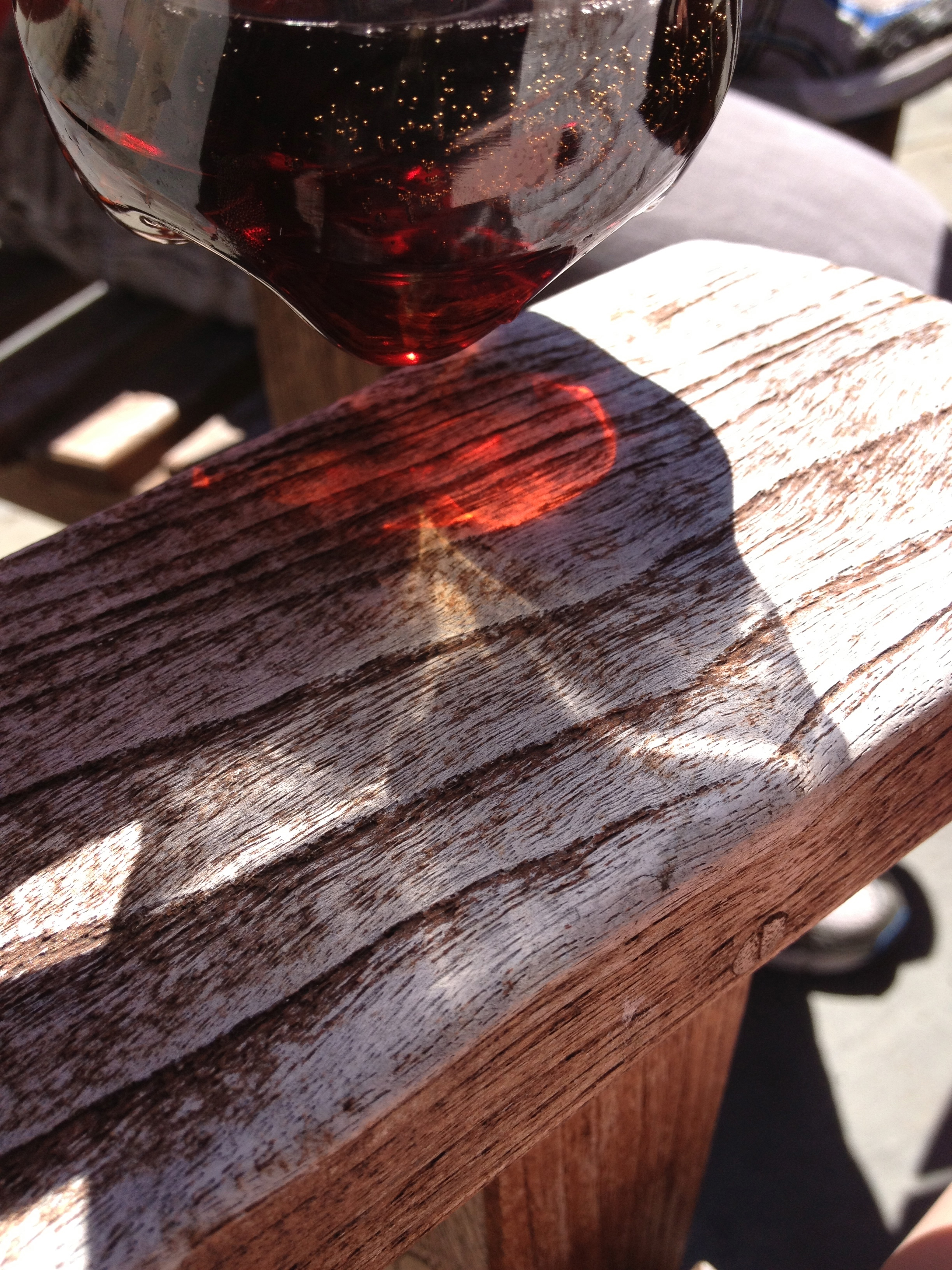
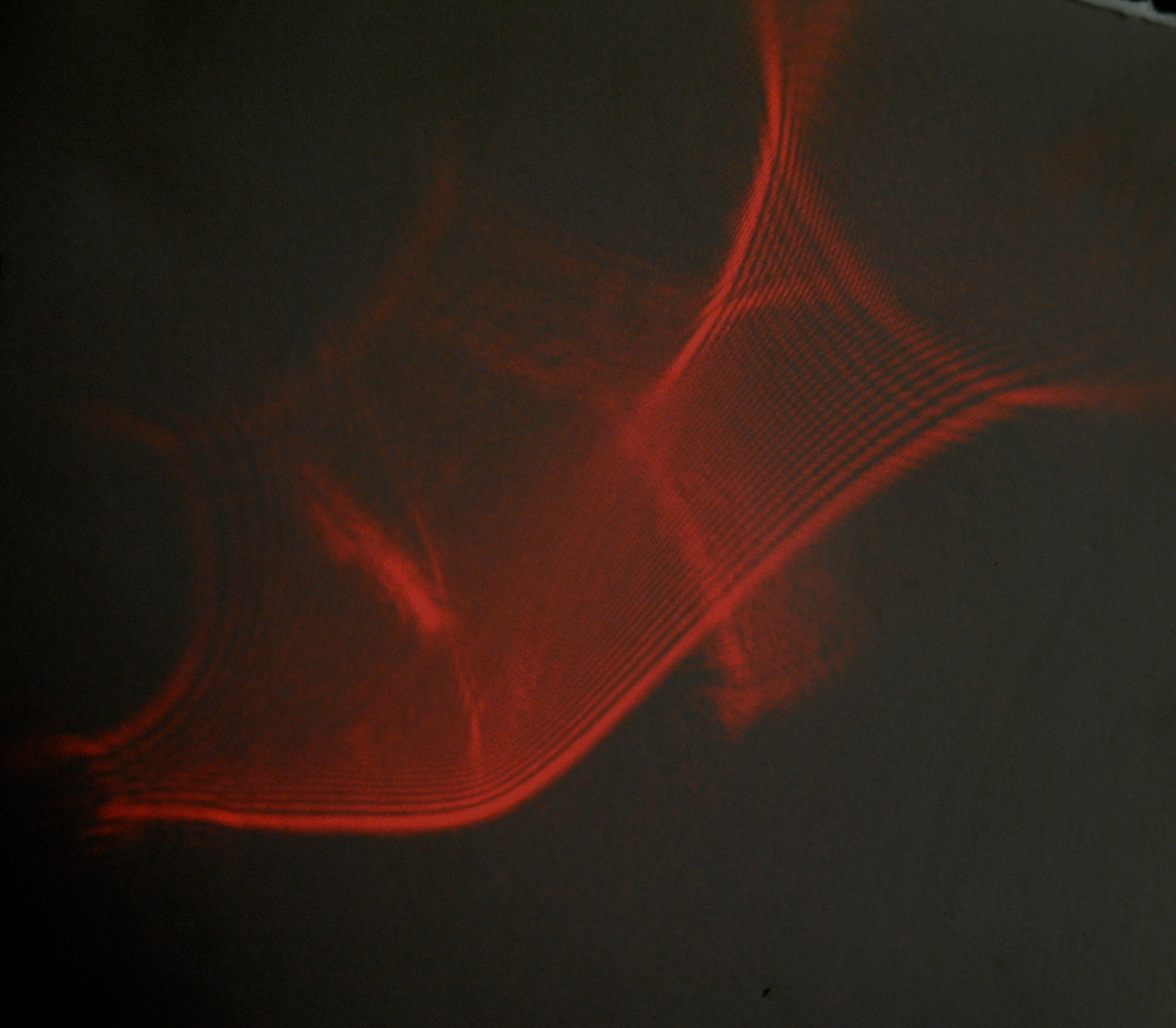
Aside from the calculus I was working on all day, at lunch I was able to
capture a few photographs and videos of caustics forming off a coke
bottle. I’ve posted a video
and a picture below. Enjoy ☺.
This morning I went straight to work. I performed three trials observing
the progression of far field caustics as the water droplet evaporates. I
recorded my observations and the time each transition took place in my
notebook. In addition, I documented each change with a picture. All of this data
can be viewed on a presentation
where
I have created a table and combined image of the caustics forming for each
of the three trails.
In the first trial the entire process took around 30min. The process in the second and third trials took around an hour.
Lock et al., describes the process taking around an hour. I believe that reason for this increased transformation time
was because of the placement of the laser beam on the microscope slide. In the first trial the laser beam was not in the
center of the water droplet, the way the slide was placed made the beam hit the bottom of drop. I also believe that the
size of the droplet affects how the caustic develops and what it looks like at the beginning of its transition. In the
first trail the droplet was larger than the others. The second trail droplet was the smallest of the three and the third
trail’s droplet was in-between.
Each transition sequence for each trail was similar in that a fold caustic was present first. Then, an elliptic umbilic
would appear and beginning to slowly merge in the fold, which slowly appeared as a cusp point, until it was completely
indistinguishable as two different features. Then, the process would reverse to just a fold until it evaporated
completely and no caustic was seen.
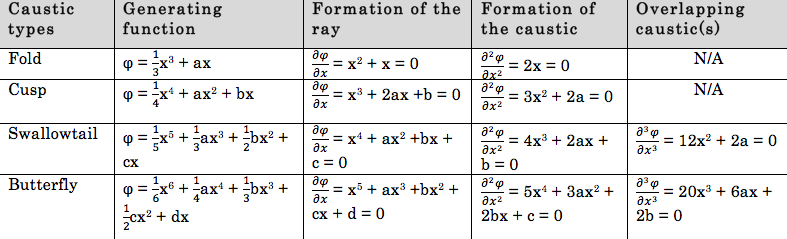
I have been exploring more of the math behind caustics. Caustics occur
when two or more light rays meet, therefore, this is equivalent to when
two or more stationary phase points join. So, caustics can be found by
setting second derivative equal to zero to find the critical points of the
map. There is a generating function that is created into standard form of
the coordinates obtained from the germ and unfolding terms. The formation
of the ray is expressed as the derivative of the generating function. The
formation of the caustic, then, is expressed as the second derivative of
the generating function. Sometimes there are overlapping caustics that are
expressed as the third derivative of the generating function. I created a
table with each of these equations for the first four elementary
catastrophes. I am still working on the last three, which have more
complex partial derivatives than the previous.
Also, today the light bulb for the microscope came! So, I made sure the bulb fit and lit up then reassembled the
microscope. I tested it out and played around with the different objectives. Hopefully I can view water droplets in the
near field with the microscope soon.
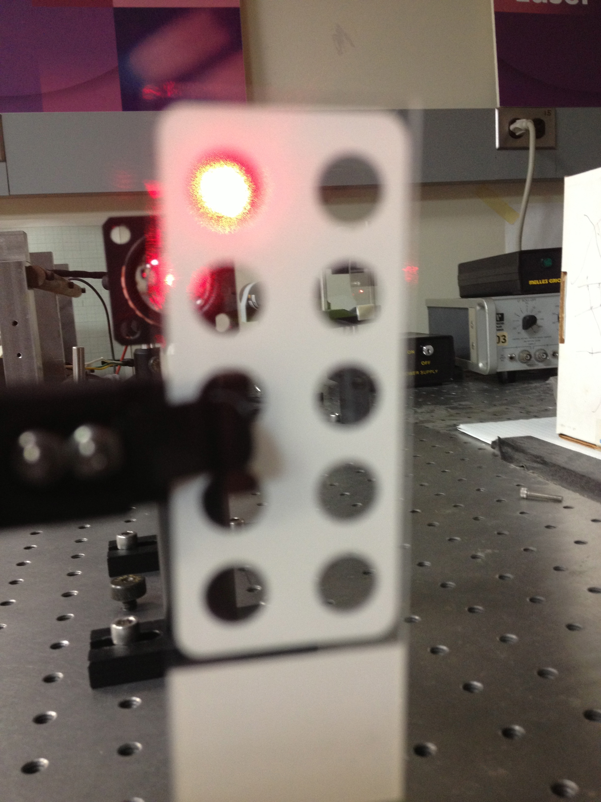
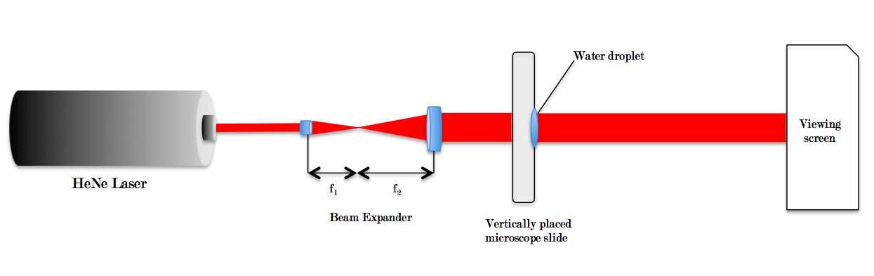
Today was a very successful and exciting day in the lab! I was able to
create a setup for viewing water drop caustics in the far field. I used a
HeNe laser and created a Kepler
beam expander. Kevin and Kathy helped me
before I began to setup, which was great. I had never really worked with
optics equipment hands on before so their help was truly welcome. Once
they explained the basics I got to work! First I began aligning the mirror
so the beam was straight (Kevin actually split the beam because he needed
the laser for his project). Once the beam was straight I created a beam
expander using two lenses in the Kepler configuration. The beam was passed
through a vertically placed microscope slide to a white form board used as
a viewing screen.
Once I had my setup I was eager to test out the experiment! I placed a
drop of water in a self-cut hole in a piece of electrical tape stuck to
the microscope slide. I immediately could see the caustics form! The water
however was absorbed through the tape very quickly and therefore the shape
of the caustic would change dramatically and rapidly. I tried using
electrical tape, scotch tape, masking tape, and this other white tape I
found laying around. The tape was clearly not working so I knew I had to
try something else. It was still amazing to see the caustics forming at
least for those several seconds.
Since the tape wasn’t stable enough for what I wanted to see, I decided to
use a microscope slide with the outlined circles that Dr. Noé found for
me. I worked really well! The droplet was stabilized and I began to see
the caustics evolve in a similar fashion to what I had read in numerous
papers! ☺
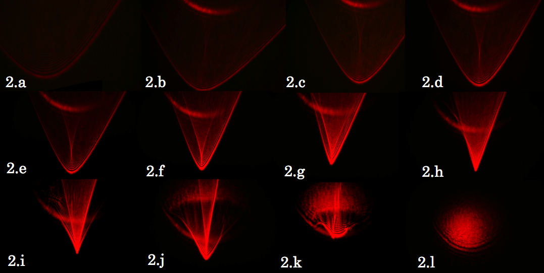
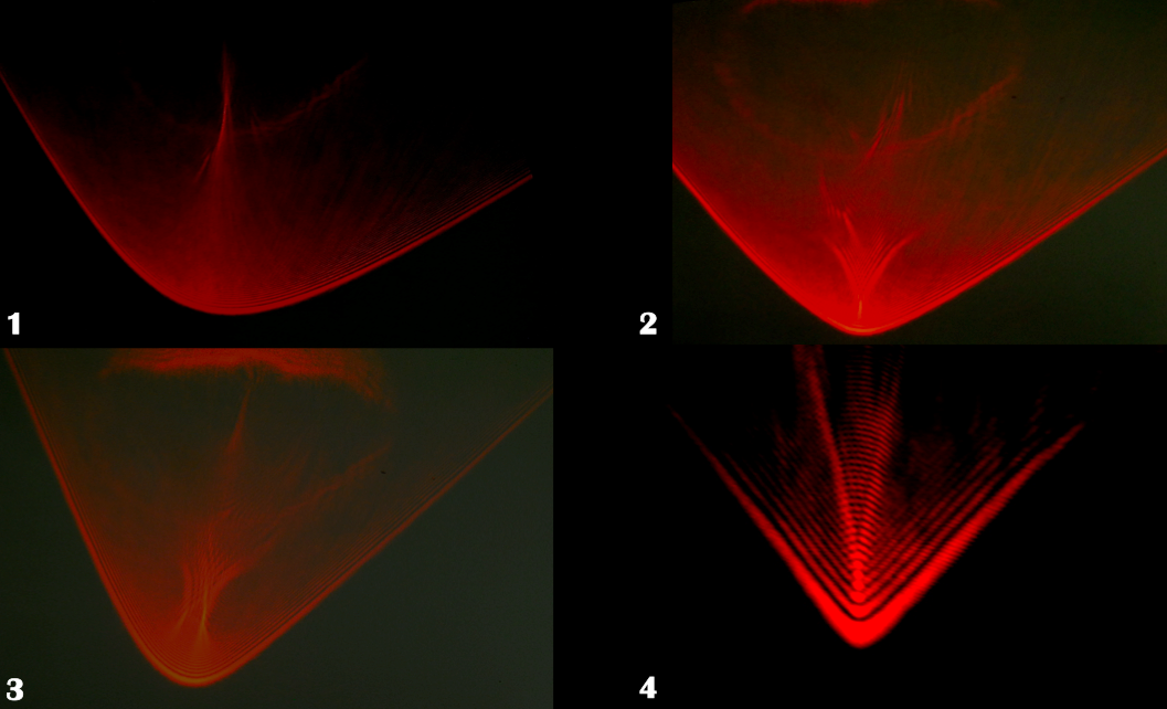
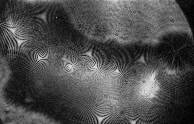
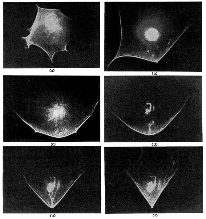
The following pictures are of the far field progression of a parabolic
umbilic caustic. You can observe different caustic shapes as the water
droplet evaporates and evolves. I have listed below the image my
interpretation of what the catastrophes are for each picture as it
evolves.
Picture 1 – fold
Picture 2 – elliptic umbilic
Picture 3 – elliptic umbilic
Picture 4 – parabolic umbilic with a hyperbolic umbilic focus
I want to point out that the evolution of these caustics is similar to
figure 1 from Lock et al. 1990. I actually have the picture in my journal;
it’s in the Friday July 12th entry. So, now that I have seen these results
in just preliminary testing I plan on replicating the set-up using the
microscope slide with the outlined circles. I plan to watch the
progression closely and record the time each transition occurs and
document it with a picture.
Today I worked on setting up a microscope to observe the water droplets. I
found an old Bausch and Lomb microscope that will be sufficient for my
project. The light bulb, however, was burnt out and needs to be replaced.
So, I spent some time taking apart the base of the microscope to get to
the bulb out. I also spent a lot of the day searching online for the bulb
and searching for a company who could deliver the bulb. After some
misunderstandings and confusing phone calls, Dr. Noé was finally able to
purchase the bulb from a local Long Island company. It should be here
Monday!
I spent time re-creating diagrams from Nye’s book of the vertical and
horizontal setups for the water droplet experiments. I actually found that
creating diagrams using PowerPoint is much more user friendly than
using Creately. The diagrams will surely help me when I begin my set up,
hopefully next week. I wondered around a little bit today and gathered
some microscopes slides and played around with setting up the vertical
microscope slide, as well.
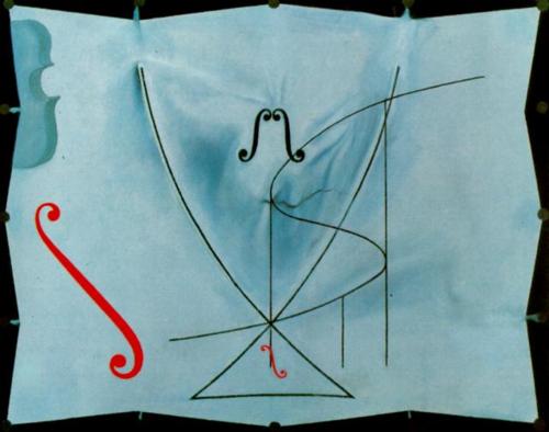
Today I also found out that Salvador Dali’s last painting was based on
René Thom’s catastrophe theory! The title, La queue d’aronde – Série
des catastrophes, in English translates to The Swallow’s Tail –
Series on Catastrophes. This painting is a depiction of one of the
seven elementary catastrophes, the swallowtail. The shape of Dali’s
Swallow’s Tail is taken right from Thom’s graph of the same title. You’ll
notice that there is also a cello hidden in the left hand corner and the
shapes of the instruments sound hole in red and black, which you could
also associate with the integral symbol in calculus.
Dali said himself that the catastrophe theory is, “the most beautiful
aesthetic theory in the world.” To me, this painting is truly a lovely
piece. It’s amazing how much science and art coalesce. I also found out I
share a birthday with René Thom! What a strange coincidence ☺.
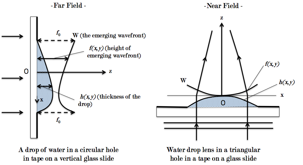
Today I explored the near field approach when observing irregular liquid
water droplet caustics. Nye’s paper describes using a water droplet a few
mm across in size resting on a somewhat clean glass plate atop a
microscope. The incident beam is parallel, in distinction from the usual
microscope condenser arrangement.
Nye was concerned with the wavefronts that are produced from a distant
point source by liquid droplet lenses whose slopes are small and which are
small enough in their vertical dimension for gravity to have negligible
effects on their shape. A water droplet a few millimeters in size
satisfies the conditions well. The top surface of the glass used is at,
say, z =0. If h(x,y) is the thickness of the drop, the height of
the wavefront, W, immediately above the drop is:
where n is the refractive index of water. There is an excess
internal pressure p of the drop which is uniform. Because of this
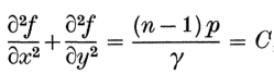
the surface tension γ causes f(x,y) to satisfy the equation:
where C is a positive constant. The Gaussian curvature is the product of
C1(r)C2(r) and can define the
curvature difference D(r) by the difference of the two functions.
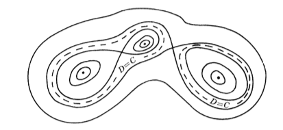
You can picture the distribution over the drop as a landscape shown below.
Just a note that at the contour D = C the line on the wavefront is
responsible for the directional caustic in the far field.
At an umbilic point D = 0, C1 = C2 = (1/2)C, and the
rays focus at the height ρ = 2C-1 above the wavefront W which
they call the focusing level F.
I wanted to figure out the setup in the papers by Lock et al. and Nye for
the
different far and near field approaches. I was attempting to create a
diagram of the far field and near field setup on Creately. I created some
rough diagrams just as a basic plan to work from. I also asked Dr. Noé and
Melia for help on what these setups would actually look like since the
papers were very vague.
At the pizza lunch today there was a talk by Giovanni Milion on vector
beams and entanglement. He explained how entanglement could be useful for
security reasons. If two photons are entangled, then if someone steals
information from one photon the other one will know immediately! After the
talk the LTC group was able to take a brief tour of ultracold lab
just down the hall. The atoms in their lab are actually the coldest
objects in New York State!
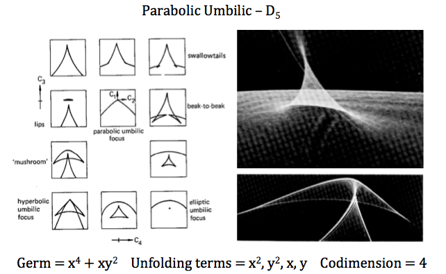
Today I created a reference page in my notebook containing the topology of
each of the seven elementary catastrophes and a picture to compare next to
each. It was really helpful because now I can look at the fundamental
equations that make up each caustic shape and the form that it actually
takes on. I was mainly interested in understanding the parabolic umbilic
form, since this is the caustic formed from water droplets in both the
near and far field.
Back at the lab I focused on understanding the caustics of water droplets
through the catastrophe theory. So, for both the far
field view and near field view approaches, the parabolic umbilic
catastrophe is seen.
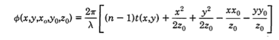
I explored the possibility of a far field approach today. Imagine waves of
wavelength λ propagating along the z-axis towards z = 0 where there is a
refracting material with index n and a thickness t(x,y).
Light refracted through this material will be observed in the far field at
points (xo,yo) on a viewing screen a distance
zo from the entrance plane.
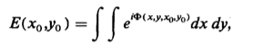
The advance in the phase of the
wave propagating from (x,y) in the entrance plane to
(xo,yo,zo) on the viewing screen is:
The optical caustic that appears on the viewing screen is determined by
the following equations. The electrical field on the viewing screen is
written as
diffraction integral over the entrance plane coordinates as:
This is just a model of what a diffraction geometry looks
like
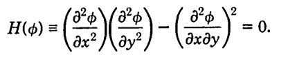
The source of the caustic is the curve in the entrance plane given by the
vanishing Hessian
Matrix of Φ:
The curve in the entrance plane is mapped into the caustic observed on the
viewing screen by the transformation:
This prescription is known as the “optical path matrix” or "singularity of
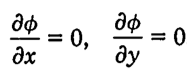
the gradient map”. If Φ is a polynomial of a low degree in x and y,
the shapes of the resulting caustics and the wave interference structure
that surrounds them may be easily calculated. In the analysis of an
evaporating water droplet it is useful that one of the properties of a
caustic is the connection between its shape and the shape of its
H(Φ) = 0 source curve in the entrance plane. If the source curve
locally resembles a line, for example, then the curve maps via the last
equation into a fold caustic.
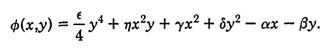
For water droplets we want the phase function for a parabolic umbilic.
This phase function of the past four equations for the parabolic is as
follows:
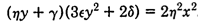
The Equation of the curve in the x-y plane of the water droplet that is
mapped to the parabolic umbilic on the viewing screen is given from the
Hessian Matrix by:
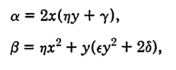
Using the fourth equation the 2D section in space of the parabolic umbilic
is given parametrically by the following (where x and y are solutions of
equation six):
With that said, if the caustic is directly observed by eye, the analysis
proceeds similarily except that Φ is no longer a function of
zo but of fo, the relaxed focal length of the
eye, and the electric filed at the location (xo,yo)
on the retina is:
where the phase function is now:
Today I also joined the Simons students to listen to a physics talk by
Professor
Matthew Dawber. He talked about Ferroelectrics and all the fun
materials he is working with on the Nano-scale. He explained the
Ferroelectric phase transitions and some of the structures used, such as
BaTiO3. They can measure the electricity by switching from a
polarization
up position to a polarization down position by electron beams. The create
these superlattice structures on the nanometer level that they observe
with an electron microscopy device to ensure these structures are up to
their standards. He’s hoping that these materials can store information,
or energy, and perhaps be used as an alternative source of energy in the
future.
Today the group discussed another estimation problem. The question
presented was the following:
In order to give a reasonable estimation I found the efficiency of solar
panels to be on average 15%, which corresponds to 150 watts per sq. meter.
I then estimated the area of the roofs of the buildings. I found that
there are 122 buildings on campus with the gross sq. fit being 10,861,402
sq. ft. Each 100 sq. ft. of the roof is equal to one roofing square ft.
So, after dividing and converting to sq. meters, I found the total area of
the roofs to be 10,090 sq. meters. The equation I used to find the total
energy was the following:
This is about equal to energy of one lightning bolt!
Over the weekend I downloaded Mathematica and found some demonstrations
where you could manipulate the shapes of caustics. I was thinking I could
do some calculations in Mathematica in the future for my project so I
started learning the basics, such as plotting functions and creating
series.
I’ve decided that I would like to create a project dealing with caustics.
They often just appear random but there is so much structure to them.
Their order is actually quite profound. They have this sharp and ordered
arrangement that forms without any preconditions, it just happens. Compare
that to high-tech efforts made to create a telescope lens; the lens focus
is unstable in that any minor agitation destroys the focus to a blur.
Unlike human focusing capabilities, caustics are truly an example of
nature’s amazing focusing power. So, I’ve been trying to come up with a
project that is feasible in the lab dealing with caustics.
This morning I explored the book on caustics I checked out on Friday. Nye,
the author, explained an experiment he performed having to do with
caustics formed from irregular water drops, I looked at his paper that
also described this experiment. He recommended that anyone with access to
a laser, a beam broadener and microscope should certainly try the
experiment because the view is just remarkable. For my project I would
like to do a setup similar to Nye’s, most like Lock et al., where they
placed a water drop on a millimeter thick screen to act as a converging
lens and used an expanded beam from a 60-mW HeNe laser to evaporate the
droplet and observe the caustics formed. This observation would be in the
far-field 2m away. Nye used the near-field approach, perhaps I could do
both and compare? Maybe I could change the diameter of the water drops I
am using to see the effects that creates? I was wondering if caustics
would still be formed if the liquid drops weren’t water, what if I used
cooking oil or vinegar?
Today I began to think seriously about what I could do for my research
project this summer. Currently, I am really interested in studying the
formation and structure of caustics from water droplets. I found a great
video that displays water drop caustics on a rainy day. They can actually
be seen forming on a lens with the naked eye.
I found a book
by J.F. Nye titled Natural Focusing and Fine
Structure of Light: Caustics and Wave Dislocations on Google books
that had a lot of information about caustics, specifically background
information about the elementary shapes and water drop caustics. The only
problem was that Google books didn’t have all of the chapters available.
So, I thought I’d try and find it in the physics and astronomy library
upstairs. Luckily they had a copy! So, I spent most of the day reading
about the amazing focusing power of light.
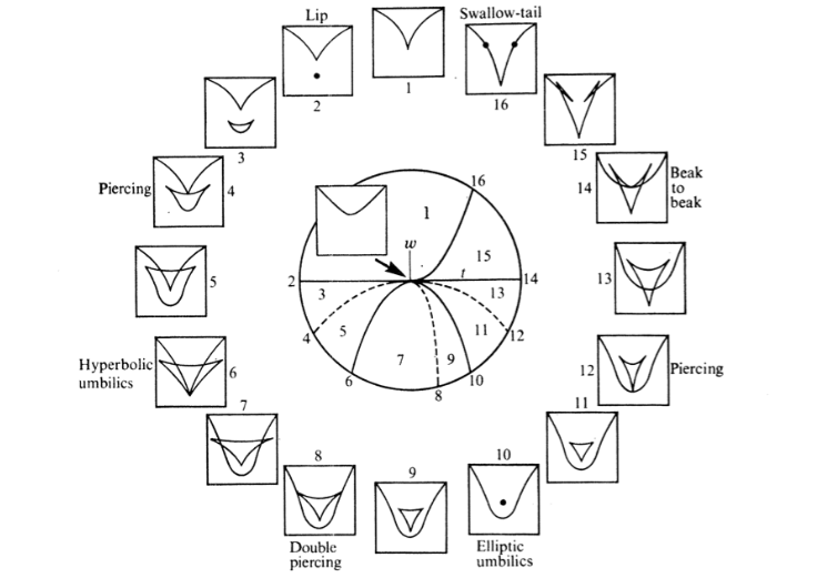
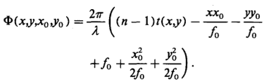
I became more familiar with the seven elementary catastrophes, or shapes,
the caustics can form into. There is the fold, cusp, swallowtail,
butterfly, hyperbolic umbilic, elliptic umbilic and parabolic umbilic. I
re-created a table that includes information on each of these below.
Also, I want to point out that umbilics, or umbilical points, are points
on a surface that are locally spherical. They usually occur where the
Gaussian curvature is positive. Their standard models are congruent with
their germ in the table (Ex: for a hyperbolic umbilic it is,
x3 +
xy2).
The table means that any potential that produces each shape, let’s use a
fold for an example, can be transformed. It can be transformed by changes
of coordinates into the standard form:
This form is for a fold, where x and y are state variables and a is a
control variable. Cusps can be transformed in a similar way:
This form is for a cusp, where there are now two control variables a and
b. The upper sign refers to the ordinary cusp and the lower to the dual
cusp. They are almost identical in all respects but have to be counted as
separate catastrophes because they cannot be transformed into the other.
The germ, which is defined as the polynomial obtained by setting all the
controls zero, contains the essence of each singularity. The unfolding
terms describe how the singularity unfolds as one moves away from the
origin in control space and their number is the same as the codimension.
Overall I think this book was a tremendous help for me. It even had a
figure showing the first known drawing of a caustic by Leonardo da Vinci!
What could be better than that? Studying these caustic effects is really
interesting because it’s been shown that similar patterns and organization
like those we see in a swimming pool explain the twinkling of stars and
they underlie the phenomenon of gravitational lensing, which makes visible
to us the most distant objects in the universe.
Today I investigated caustic architecture by reading blogs, papers, and
watching videos by a group that makes images come to life just by playing
with light. Their goal was to take random caustic effects and control them
into almost any desired shape. To design such a image, or caustic image as
they say, one would need to solve the inverse problem. They created an
algorithm that combines the requirement of an integrable normal field with
the goal of reproducing an arbitrary intensity target image by the caustic
created through the reflection or refraction of the computed object. What
is created (for a refracted image at least) is a large, transparent plate
capable of generating a high-resolution image when a light is shone
through it.
This idea of creating images based on caustics really intrigued me. At
first I read a general paper this group had written on the general
properties of these caustic images. It didn't explain the optization
algorithm and referred me to a technical paper. Unfortunately, I could not
find this technical paper anywhere. I did a little more digging and found
an earlier paper the group had written that explained some of the math
used to make these Gaussian kernels that projected the image.
I wanted to see if Dave or Sam knew anything about these caustic
images so I showed the video to them, they were both really
amazed. They hadn't seen anything like it before. Dave told me it reminded
him of scratch holograms which you can easily make at home with a few
simple supplies. After investigating how to make scratch holograms
I realized this could be a really great mini project in the LTC!
Laser Sam also gave another presentation today; this one was about laser
safety. Basically vision damage and electric shock are the two main safety
issues that we should be aware of in the lab. There are other hazards too,
such as chemicals from liquid lasers that have toxic dyes. He talked about
the different classes of lasers and the dangers of each type as well. One
of the main lessons I took away from the presentation is that having
better work habits is often better than worry about what type of safety
goggles to use.
I read another paper
today about caustic effects due to sunlight.
These
“death rays” (aka reflections from curves) reflecting off large buildings
are become hazardous to people. So, the building is made of shiny,
reflective surfaces with reflection coefficients well above those from
normal untreated glass. The reason they do this is to prevent an intense
thermal load inside the building during the summer. But, as a consequence,
a much higher percentage of the incident light is reflected, which can
cause disturbing and blinding light spots. Guests of one Las
Vegas hotel complained about the intense heat saying that their hair felt like it was
burning and their plastic cups were being melted! That’s the power of
light for you!
Today Laser Sam
gave his presentation at the pizza lunch on lasers and the
LTC group gave mini presentations on their progress so far. Sam talked
about the basics of lasers and the different types of lasers that are out
there. I learned that solid-state lasers were the first ones to be
invented and gas lasers were actually second. He focused in on
longitudinal laser modes and how to analyze the gain curves with the
scanning Fabry-Perot interferometer. Hearing Sam’s talk, followed by
Casey's, Rachel's, Stefan's, Kevin's, William's and Kathy’s talk, I really
was able
to get a better grasp on all of the projects taking place in the LTC. I
definetly have learned more about lasers in this past week than I thought
was possible! I
also presented a powerpoint on my progess so far.
A lot of the physics pieces I’ve been picking up over the last week are
clicking into place!
After our lunch/meeting I was able to take a tour of Dr.
Eden Figueroa’s
quantum computing lab. In his lab they are working on creating a computing
device that works on the quantum level. So instead of using a light beam
with many photons they want to harness a single photon to transfer
information. He used a really great analogy that made it easy to
understand. Think about trying to find out the information on several
streets off of a main road, such as the types of houses, trees, etc. that
are on those streets. You would have to go through one street to obtain
that information and then come back to where you started and go to the
next street and on and on. If you were a photon, however, quantum
principles make it so you could be in on all those streets at once! He
showed us the lasers he uses and some of the experiments that are
underway. I definetly couldn’t grasp all the concepts fully but I love
thinking about quantum physics, it has always intrigued me ☺.
In between the talks and the tour I read a paper that
explored
experiments
with the topology of caustics using nematic liquid crystals. Which
combined the primary topics I have been studying for the past week! In
their first experiment they produced biperiodic caustics by defecting a
light beam through a nematch liquid crystal layer. This setup was used to
check the topological constraint expressed by the Chekanov relation. The
experiment produced a virtual part and real part of the caustic.
The expected value of the umblicis is 0, four real (elliptic)
umbilics D4− , and four virtual (hyperbolic) umbilics D4+. Basically
the correct number of umbilic types were observed and corresponded
correctly to the Chekanov formula. They also had an interesting point
towards the end of the second section. It would be interesting to find out
if other caustics exsist with the same biperiodicity, but with a different
number of umbilics (per unit cell). Moreover, it would be interesting to
see if you can obseve a caustic without any umbilic. The possiblity is
theoretically allowed but has not been experimentally checked up until
their paper.
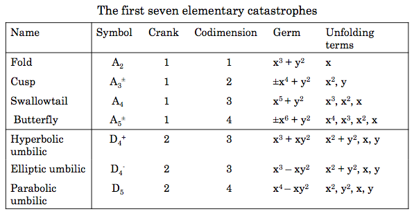
Today I read a paper
on measuring distances based on caustics. Illuminating an ellipsoid mirror
by a point of light formed caustics and two techniques were employed for
range finding. In technique A a reference
screen was placed far away from
the mirror and in technique B a light
source
was placed far away from the
mirror.
The point source is denoted as K and the screen is denoted as Sc. The
correct position of the second point M' can be derived and checked from
the shape of the caustic on the screen. The caustic depends on the
particular form of the ellipsoid mirror, defined by (a/b) of its principle
elliptic axes, as well as on distance A of the point light source
illuminating the mirror. The caustics are formed at various distances
(A/b) and the distance under measurement can be evaluated as the mean of
all distances defined by the corresponding caustics.
Technique B was found to be more favorable
over technique
A because the
caustic is formed on the reference screen near the mirror therefore it is
better illuminated than if it were formed on a remote screen in the first
method. So, it was concluded that large distances could be measured
without the necessity of running these distances.
I also decided that today I should research lasers and get a better
understanding of the other projects that are starting in the LTC this
summer. Coming here I didn’t know much about lasers and just did some
basic research prior to starting. So, today I decided to explore Laser
Sam’s website, which contains basically everything you need to know about
lasers. He had great information about the basics of how lasers work.
There was a really great diagram on the basic laser
operation that really helped me visualize the lasing process. It was also
really helpful to read about all the specific terms and names that are
associated with lasers (such as the HeNe laser’s common “Hee-nee”
pronunciation) so I can follow along better with students in the lab. Now
when I hear someone talking about Fabry-Perot
resonator I’ll know exactly what he or she means☺.
I was reading a section on diffraction gratings
on Sam’s website that
caught my attention; mostly because of the idea that 3D glasses from a
cereal box can be used as a diffraction grating. Usually I only think of
CD’s or DVD’s having this property. As I started to think more about the
3D glasses being used as diffraction gratings I started to think about
another type of 3D-like glasses I had as a child at Christmas time. I
would put
them on and
look at the lights on the Christmas tree and see little snowman where each
point source of light should be. It was neat to make the connection to the
glasses I had as a child and the
physics behind them.
I tried to do some more research to find out how exactly
these images are formed. I couldn’t find any specific answers. I do know
that the polarization of light effects what the eye sees and therefore
with the right type of covering all types of interesting lighting effects
can be seen. A diffraction grating will split and diffract light into
several beams traveling in different directions. The directions of these
beams depend on the spacing of the grating and the wavelength of the light
so that the grating acts as the dispersive element. Spectroscopy has a
special place in my heart as well, so I am interested in the idea using
diffraction grating to check the wavelength of a laser. Now that I have
the basic understandings down I am excited for Sam’s talk (well I guess
small individual talks) on lasers tomorrow at the pizza lunch!
Laser Sam arrived today! The group went to the Simons Center for a
delicious lunch in honor of his arrival. Back in the LTC I switched gears
from caustics to topological defects and their structural formation. I
read a few papers on the dynamics of this really interesting effect. As I
mentioned in an earlier journal entry, these defects are believed to have
formed during phase transitions in the early universe. These topological
defects carry energy; this energy leads to the attractive gravitational
force. Therefore, the defects can act as seeds for cosmic structures. I
read that these same transitions that are believed to have occurred in the
early universe can be seen in liquid crystals (the same principle I read
in several other papers).
In particular, one paper I read on the dynamics of topological defects in
nematic liquid crystals was very interesting. They described their
research on investigating the annihilation dynamics of defects and
antidefects in lyotropic nematic liquid crystals (a mixture of potassium
laurate, decanol and deionized-destilated water). Something they claim has
not been done before. They analyzed Schlieren textures using a polarized
optical light microscopy. The nematic phase is the most known
liquid-crystal mesophase. The liquid-crystal nematic mesophase and the
isotropic phase can be characterized by the birefringence (Δn); Δn ≠ 0 is
a liquid crystal in the nematic and Δn = 0 is the isotropic phase. The
nematic phase can be obtained by decreasing the temperature from the
isotropic phase. Due to the birefringence of
the liquid-crystalline
mesophases, and their small elastic constants, they are ideal materials to
study the defect dynamics experimentally. Below the first image is
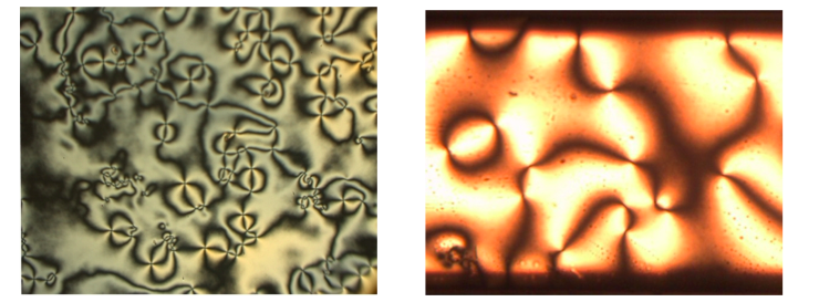
Schileren texture of a thermotropic liquid crystal after the
isotropic-nematic transition. The second image is of Schileren texture of
a lyotropic mixture.
For their experiment: There was a sample placed in a glass capillary with
100μm light path. The borders were sealed with a paraffin film followed by
a nail polish coat in order to avoid changes in the mixture concentration.
An analysis between crossed polarizers in an optical microscope (5x
objective and 10x ocular) connected to a CCD camera was conducted. Using a
hostage with a X-Y micropositioner connected to a computer controlled the
heating and for the cooling they used a water bath. The first glass
capillary was 25°C and then the temp went up to 50°C in order to reach
isotropic phase. In order to obtain desired phase around 40°C they reduced
the temperature to 25°C. After about 5 hours the topological defects were
pronounced and visualized by the CCD camera.
This morning the group discussed an estimation problem, my first
estimation problem here at the lab. The question asked was, “What is the
maximum angular resolution of the human eye?” When Melia emailed me the
question a couple days ago at first I was stuck. But, as I thought about
it more (and realized we could use the internet to lookup physics topics)
I had a better sense of what I was doing. I was able to find the physics
equation for angular resolution.
Once I had the equation I began estimating numbers to plug in. For the
wavelength (W) I plugged in 510nm, which is green light. For the diameter
(D) I estimated the diameter of the human eye to be 5mm. After plugging
in the numbers I got .007 radians. While my answer is not the correct
answer (which I looked up online after and found the answer to be 4
arcminutes or .001 radians), it was the process that really mattered to
me. All of the group’s answers were pretty close and thinking about how
each of us got our answers was a really neat process.
Today the group also met in the conference room where I showed them
how to install and use Python to plot data. I described software you would
need for different platforms and showed plots of sin functions and modest
3D galaxy model. The group stayed in conference room to look up articles
as a group on the American Journal of Physics and Optics InfoBase. I'm really
glad i was exposed to these resources and I used them later in the afternoon to find some really interesting articles.
Back in the lab I hunted around for additional scholarly papers on caustics and their properties. I read a paper on the caustic surfaces of a refractive laser
beam shaper. Basically they proposed that understanding the caustics of beam
shapers and how wave fronts interact with caustics will lead to a greater
understanding of beam shaping and will improve it as well.
I also read a paper on caustics formed from evaporating water drops. This was really interesting and
it was a paper that really connected a lot of what I had been reading about caustics, especially the very math-based catastrophe theory which is based on
diffraction. The paper describes the process of how caustics evolve on an
evaporating water droplet. As the water slowly evaporated the caustic at the bottom
of the viewing screen come to dominate the entire field of view and its shape evolved into the diagrams shown below.
Lastly, today I found an awesome picture
on the Optics Picture of the Day (OPD) website that shows rapidly moving caustics at the bottom of a stream
and the distortion of a trout caught by the caustics!
Today I continued searching for possible research topics. I began by reading a paper
on the properties of optical caustics in nature. They described the effects made by a drop of water and a
rainbow. They provide a diffractional integral approach that they find a simpler method for explaining and
analyzing the caustics formed by natural phenomena.
I explored the effects in liquid crystals today as well. A paper on the lensing effects in a nematic
crystal
caught my attention. First I wanted to find out just what exactly a nematic crystal was. I learned that
these crystals are s state of mater that has properties in between those of solid and crystal. The word
nematic actually means, “thread” in Greek. It has fluidity similar to that of ordinary (isotropic) liquids
but they can be easily aligned by an external magnetic or electric field. These nematic liquid crystals are
commonly used in LCD displays.
The article describes topological defects (or disclination) in the crystal. These defects are believed to
form when symmetry is broken into a phase transition. What really grabbed my attention reading this article
was its connection with cosmic objects and gravitational lensing. Objects such as cosmic strings change
their topology and, therefore, introduce interesting phenomena like gravitational lensing.
Today was my first official day in the LTC! I spent my time in the morning
researching possible research topics. In preparation for this program I
did a little reading up on gravitational lensing so I decided to start
there. I wanted to find a source that could connect gravitational lensing
to something I could accomplish in the lab. I found a great site that
talked about geometric lensing. The essay describes a 2D cone that can be
slit along the side at a drawn line (think about it as a light ray) and
placed flat. It shows that the object can be seen at each edge of the flat
cone. It demonstrates that two light rays can appear to be originating
from two objects, one on each side of the singularity of the cone. This
doubling effect is the 2D form of geometric lensing.
I then explored geometric optics and optical aberrations, which then led
me to caustics. At first caustics intrigued me because I remember hearing
a talk by a graduate student at RPI who was studying dark matter caustics.
I began researching caustics more in depth and found a paper by M.V. Berry
that discusses the diffraction patterns of caustics later in the
afternoon.
There was a pizza lunch today, which I presented a presentation at. I
talked about my experiences as a high school student researching and all
the opportunities I had available to me. I also discussed some of the
astronomy background of my research and some of my actual research. I had
a great time speaking to everyone and responding to everyone’s questions.
Presenting my research is actually one of my favorite parts about
researching besides the actual research.
After lunch the LTC group stayed back to have a meeting discussing the
progress of everyone in the group. It was great to hear what all the other
students are interested in researching. Dr. Noé also brought in some old
science books. One of which was an astronomy book written by William
Herschel! That was pretty exciting. It was also really awesome to see some
of the laser setups in the lab. In my previous research I was staring at a
computer screen for the large majority of the time. I can’t wait to become
apart of a more hands on research experience!
Thursday August 1 2013
Wednesday July 31 2013
Tuesday July 30 2013
Monday July 29 2013
Friday July 26 2013
Thursday July 25 2013
Wednesday July 24 2013
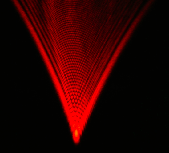
![]()
Tuesday July 23 2013
![]()

Monday July 22 2013
Friday July 19 2013
Thursday July 18 2013
Wednesday July 17 2013

Tuesday July 16 2013

Monday July 15 2013
Friday July 12 2013
Thursday July 11 2013

Wednesday July 10 2013

