
I'm back home in Minnesota now. Last Friday, August 9, was the last day of the Simons program. We had a poster symposium in the morning, the closing ceremony right after, and a lunch at the Simons center with the lab group. After lunch, I stopped by lab one last time to say goodbye to everyone (and my laser) before packing up and catching my flight home. I'll really miss all the connections, friendships, and experiences I've made this summer. Thank you everyone who was a part of it.
The poster symposium went well. I felt I was able to explain my project nicely to other students and parents. Many of them told me that they actually understood my project after I explained it (unlike some of the other projects). I suppose the Simons tour of the LTC helped out.
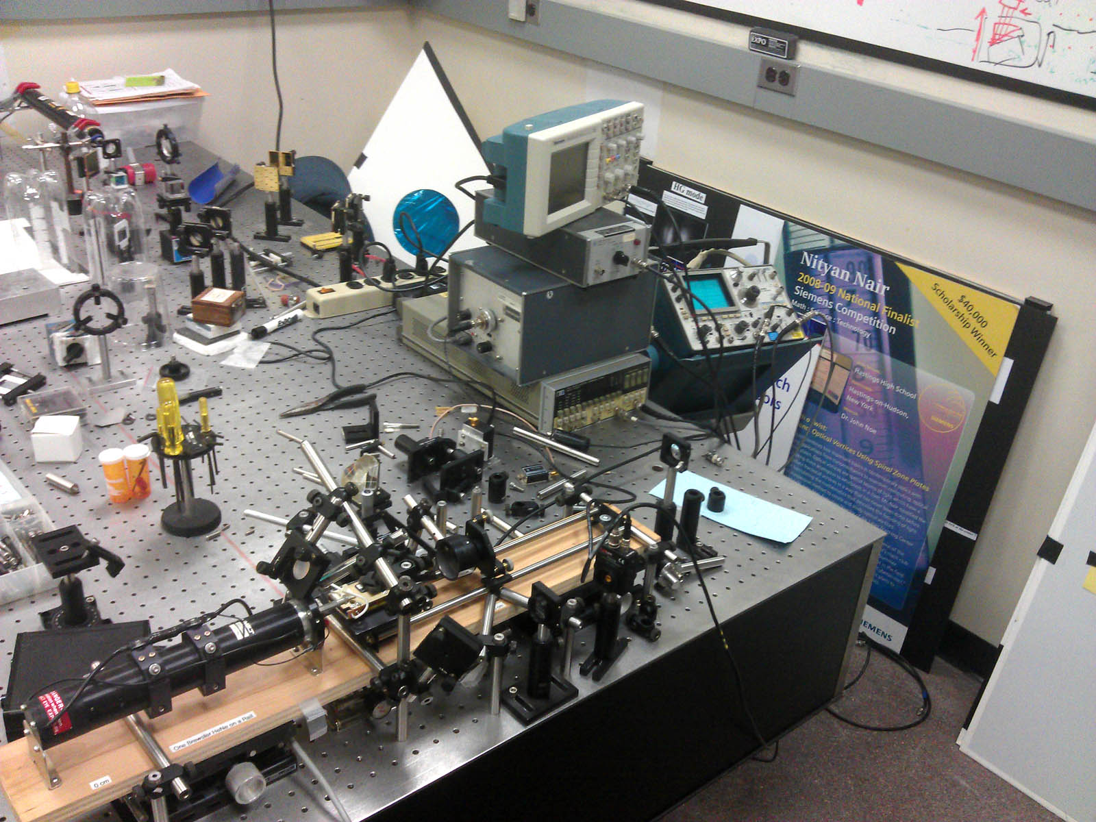
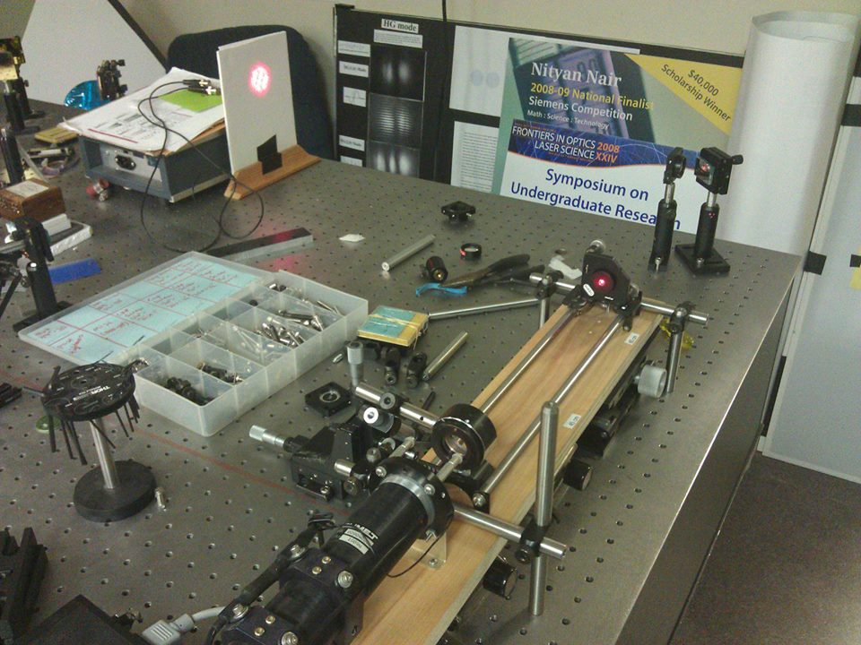
I'm pretty into photography, so I also took some time to take some nice photos of my setup last Thursday. Here's a photo of me and the laser. Click to enlarge. I'll have some more soon.
The laser beam is visible solely because of scattering in the air (not digital manipulation). For those who want to know, this was a 3.2 second exposure at ISO12800 and F11. I chose narrow aperture to get the point-star effect (a polygon diffraction pattern!), and the high ISO to minimize the shutter speed (so I wouldn't have to stand as still). The focal length was an ultrawide 16 mm equivalent. Noise reduction and selective exposure adjustment (darkening the edges) were performed in Photoshop. The original is pretty ugly.
I was pretty busy earlier this week getting my poster and abstract finished. Now that everything is finished, here's what's been going on laser lately:
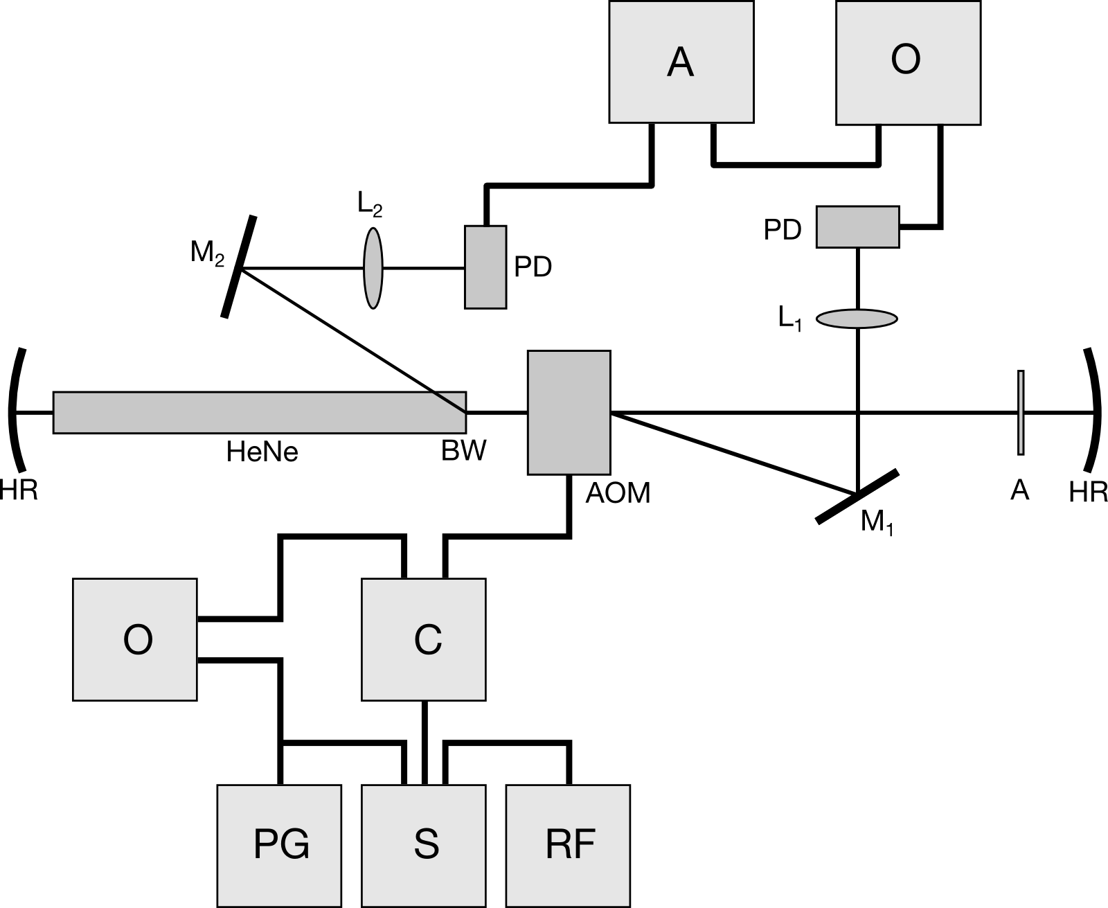
HR, high reflector; HeNe, helium neon tube; BW, Brewster window; AOM, acousto-optic modulator; A, aperture; M1, clipping mirror; L1, 75.0 mm lens; M2, mirror; L2, 25.4 mm lens; PD, high speed photodetector.
A, amplifier; O, oscilloscope; PG, pulse generator; RF, RF oscillator; S, RF switch; C, RF coupler.
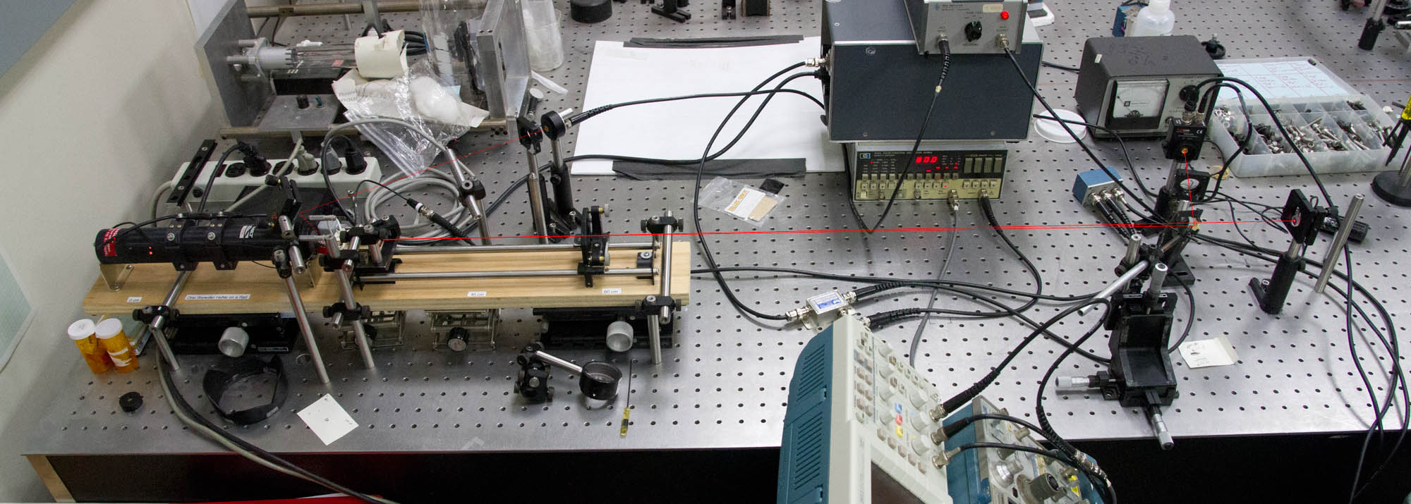
Click the image above to enlarge it. The HeNe tube is on the left, and the laser beam paths are traced. This is before the AOM was moved to the beam waist.
The lengthened cavity is 1.42 meters long. The high reflector in the HeNe tube has a 0.45 m ROC. The free standing HR has a 1.0 m ROC. Gaussian beam calculations show that the beam waist is about 1 m from the 1 m ROC mirror. I moved the AOM to this location such that the light interacts with less of the AOM optical medium. Circulating power visibily increased.
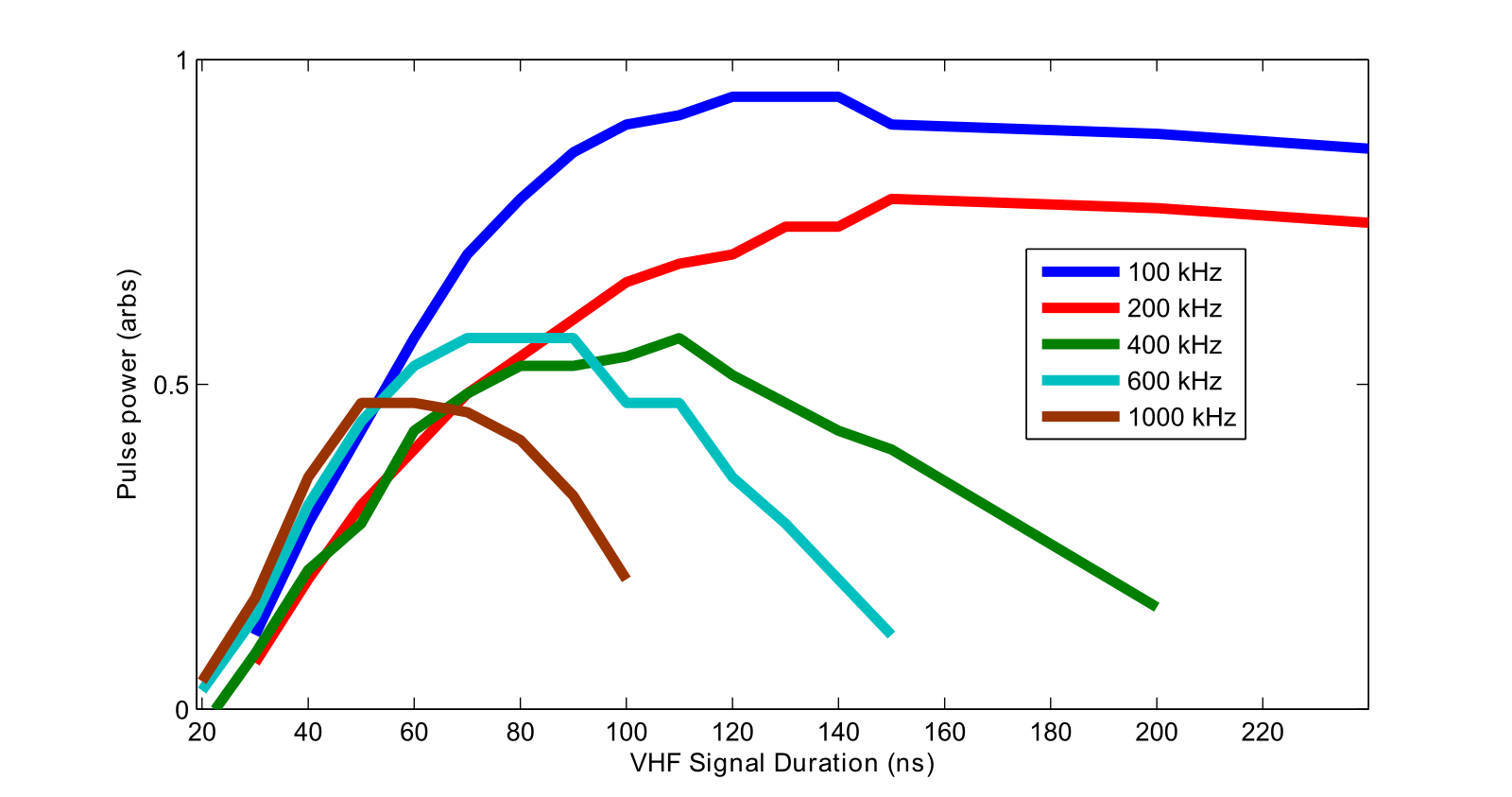
To characterize this, I tested the AOM accross repetition rates of 100 kHz to 1 MHz, and AOM on times 20 ns and up. I used the 64-trace average from the digital oscilloscope to record the pulse duration (fwhm) and peak to peak voltage of each pulse. This gives information about pulse duration and peak power (recorded photodetector voltage is proportional to peak power).
Pulse duration is consistent, between about 90-110 ns. I have not analyzed for trends here yet.
Peak power, as expected, is low when the AOM on time is low (20 ns), since the AOM is not on for long enough to sufficiently dump the cavity. Peak power rises and hits a maximum for a certain AOM time. This is when the AOM is on long enough to cavity dump the pulse, and off long enough to allow power recovery. Circulating power may not go to zero or reach its maximum. For low repetition rates (eg. 100 kHz), the AOM can be on for longer periods of time while still maintaining high peak power because there is sufficient time between the time the AOM turns off and the time the AOM turns on again to fully recover the power.
Today, I also tried collecting more data. I took photos of the 64-trace average on the digital oscilloscope and collected peak to peak powers and pulse durations for various repetition rates and AOM on times. However, something very peculiar happened: There seemed to be two-peak pulses forming. I had no idea what these were, nor did Marty. I might ask Marty to try testing the system out again after I leave to see if this still persists.
t seconds after AOM on, for one-pass AOM efficiency η, cavity length L, and initial power P0.
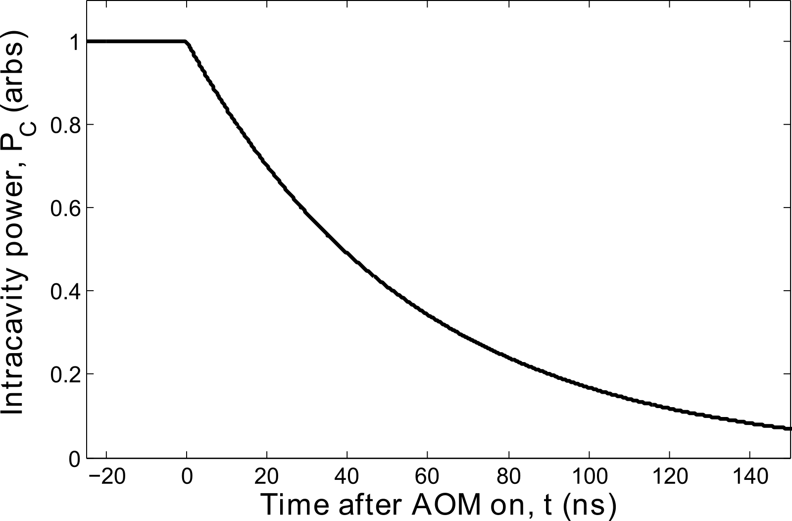
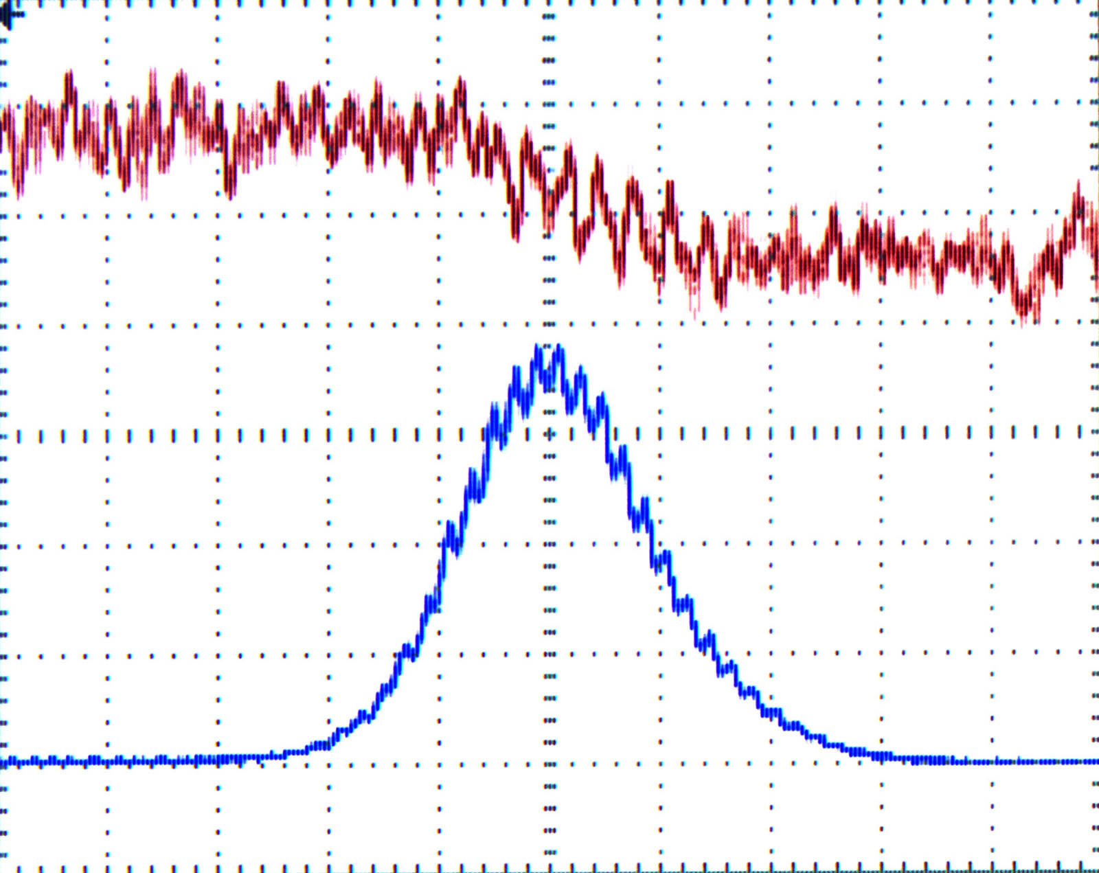
The 64-average traces above are intracavity power (red) and laser output (blue) while operating at 300 kHz. The time scale is 50 ns/div. It initially puzzled me as to why each pulse was so symmetrical. From the intracavity power calculations, we can see that instantaneous ejected power starts high, then decreases gradually. I thus expect the pulse to sharply increase in power, then gradually decrease. In the actual pulse shape, we see that the pulse is pretty symmetrical. Why?
After a discussion with Marty, we determined that the finite rise time of the RF signal (about 25 ns), and the gradient (rather than binary) cross section of the beam caused some smoothing of the pulse shape. In the example above, you can see that the rise is slightly steeper than the fall.
The modulation within each pulse (and in the intracavity power) has a period of about 10 ns. This is consistent with the c/2L mode separation beating inside the cavity. I thought it was pretty neat that we could observe this inside our pulses.
Over the past few days, I've been digging through the box of laser mirrors for heium neon high reflectors. HeNe mirrors are blue/turquoise when viewed head on, and you know you've found one when you look through it and the red from a HeNe laser disappears. Most of the mirrors were planar, or had a 1 or 2 meter radius of curvature. For laser resonators to be stable, 0 < g1 * g2 < 1, where g = 1 - L/r, and L is the resonator length, and r is the radius of curvature of the mirror.
The mirror installed in the tube has a 45 cm radius of curvature. The stability calculations reveal that with a 1 meter radius of curvature mirror, cavity lengths between 1 and 1.45 meters are stable. Unfortunately, this distance was off the table, so I got an optical rail and some long posts to extend the table a bit. I screwed the 1 m ROC HR in an adjustable mount at about 1.3 meters, and after a few minutes of alignment, got it lasing!
It was really quite impressive to see so much circulating power (>1 watt) in such a long cavity. Even with the lights on, the beam was clearly visible. With the lights off, it was even more impressive.
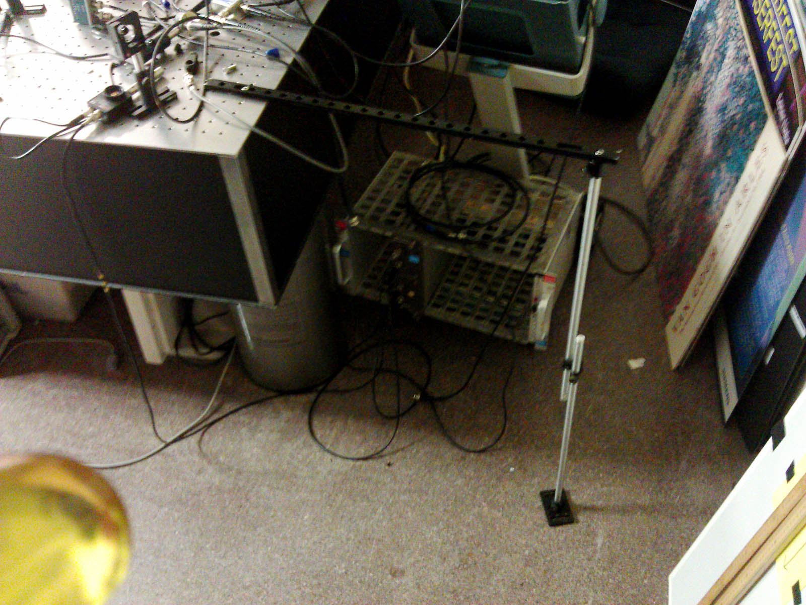
The setup was pretty unstable, unsuitable for my goal of picking off the cavity dumped beam. Although it lased with no problem, it would be too inconvienent to actually do anything with it, since the free HR was mounted so precariously. Because a longer cavity would be the only way to extract the deflected beam from the AOM (which deflects it by not a lot), I decided that I would move the entire setup to the long edge of the table. Although it looked like it would take a while, I got it done pretty quickly.
With the new setup, picking off the deflected beam is very easy. I'll be looking at the signals in the next few days.
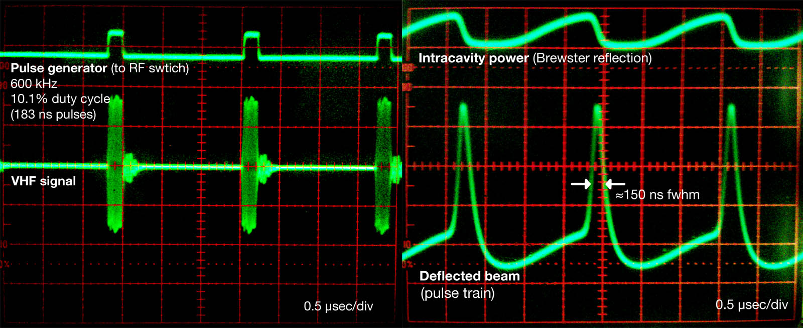
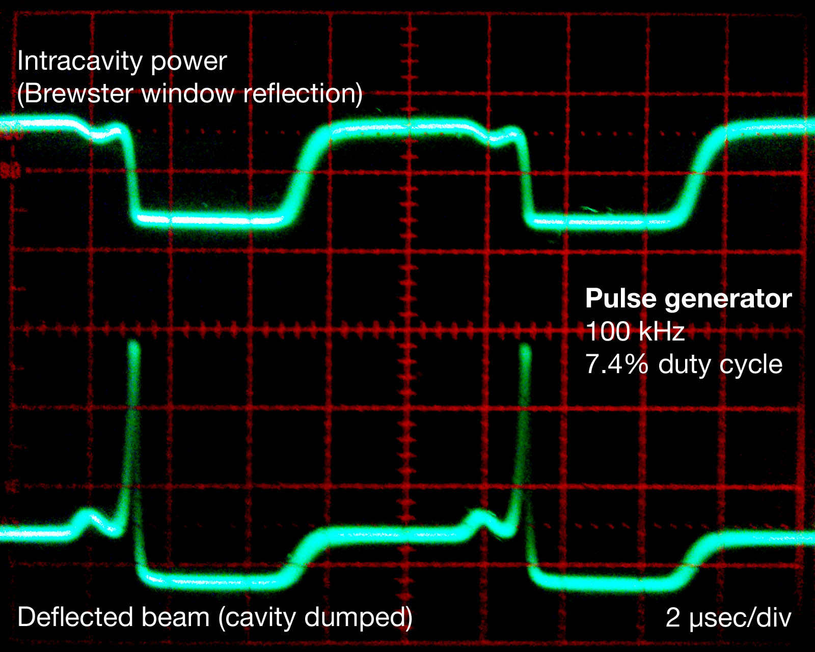
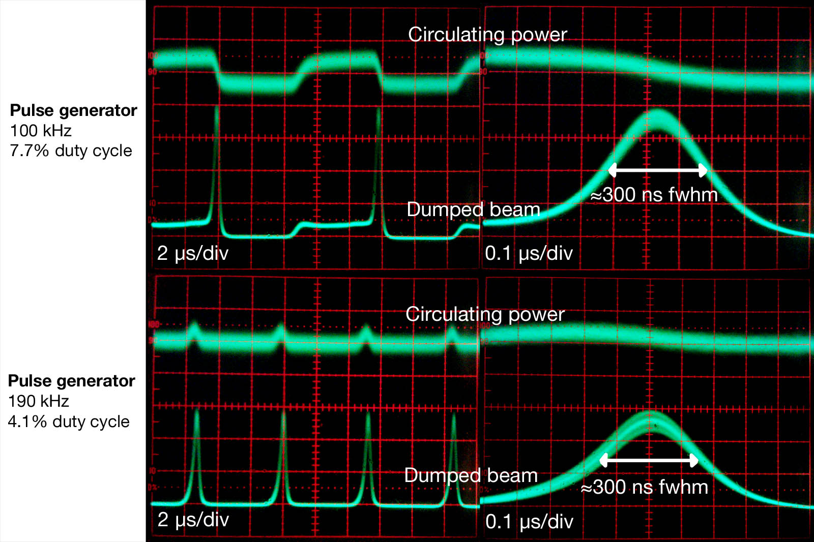
I played around with the pulsed laser light today and did some qualitative characterization of the laser and VHF pulses.
Constant at div -1.5 to 0.5: Circulating power reaches a limit, and does not get any higher. AOM off, waiting to turn on.
Peak at div 1: ??? - See VHF pulse characterization. (AOM on?)
Peak at div 1.5: Dumped pulse, under 300 ns fwhm. This corresponds with the drop in intracavity power (top trace drops off sharply). AOM on. Note that this is less than 1/4 of the power being deflected (as the AOM, as positioned (centered) deflects to 4 first order beams, two in each direction), and much energy is lost as the pulses hit to mirrors and go through a lens.
Lowest point at div 1.5 to 3.5: All circulating power dumped. AOM on, waiting to turn off.
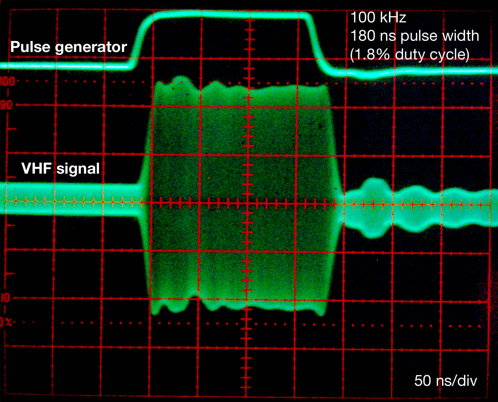
Marty realized a problem with my setup: I had T'd off the VHF oscillator so I could monitor one channel on the oscilloscope, and send one to the AOM. This caused some reflection, and because the two signals were not a copy of each other (due to different destination properties), what we were seeing on the oscilloscope was not what the AOM was receiving. To remedy this, we used a direction coupler to send a copy to monitor on the scope.
What we saw was not very good. Though the specifics of the shape of the pulse changed slightly, the overall shape was still not good for pulsed laser operation. The length of the pulses was much longer than the input pulses, and the cutoffs were not clean. This applied to pulses at any repetition rate: The modulator was too poor. A <1 μsec pulse from the pulse generator turned into a multi-microsecond VHF 'pulse' with a moderately sharp rise and gradual falloff to zero. We determined that this was probably what was causing the irregularties of the laser pulses.
To solve this, we used a high speed RF switch. This device takes in a cw VHF signal, and modulates it such that the signal passes through when a pulse is on, and turns it off when the pulse is off. This switch works much better than the internal modulator, which is only spec'd to 100 kHz (and in practice, is really poor at it).
The VHF signal look a LOT cleaner with the switch, although the signal to noise ratio isn't as good. The pulsed laser output also doesn't have the weird features anymore. I'll be looking more throughly into this (and other switches) tomorrow.
The amplified photodetector arrived today, so the first thing I did was try it out with the HR waste beam and the Brewster window reflected beam. The signal was not as strong as I would have liked (it was on the order of tens of mV), but the fall time was definitely observable. the Brewster reflection/HR waste beam fall time corresponds with the cavity dumping itself, which gives us pulse duration. This was on the order of several hundred nanoseconds. I haven't looked into this extremely throughly yet though.
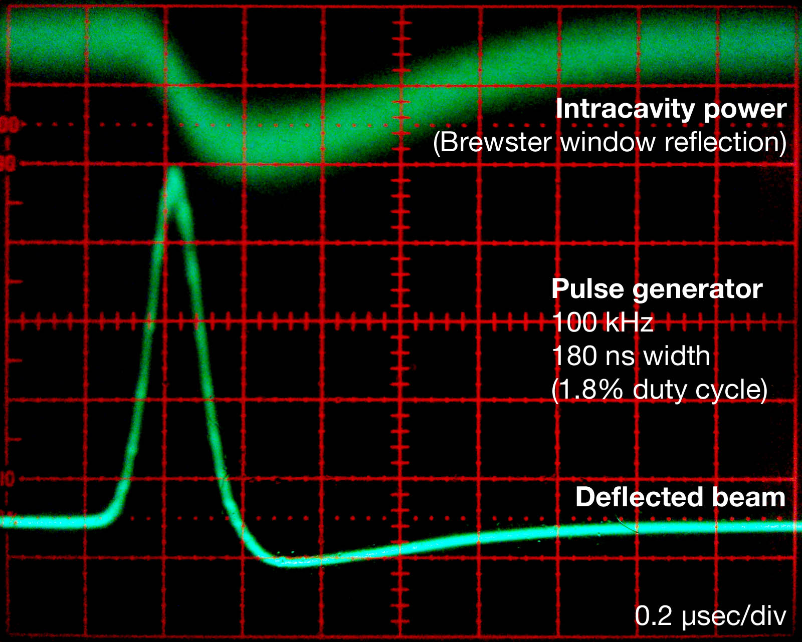
In addition to looking at the intracavity power (via the Brewster window), I also tried to deflect some of the beam out of the cavity, mid cavity. I did this by placing a 1/2 inch circular gold mirror on an edgeless mount about 6 or 7 cm away from the AOM and fiddling around with it so that it just barely scraped the edge of the intracavity beam. The deflected beam looked fairly bright and was bounced off another mirror then focused onto the amplified photodetector. The idea was to try to extract the (very narrowly) deflected beam, and accept a bit of circulating intracavity power with it. I used an aperture to clean the beams to TEM00 as well. The pulse generator was set to 100 kHz, 9.26 μsec pulse width.

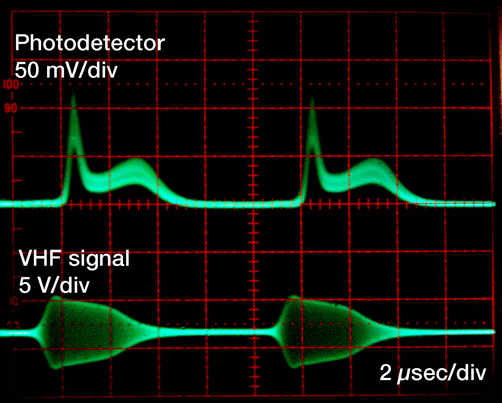
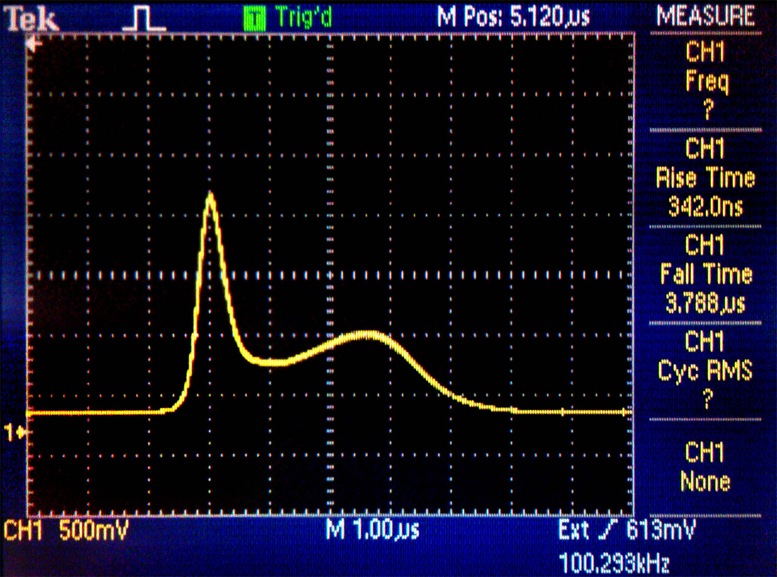
I connected the photodetector to the digital oscilloscope and displayed the running average over 128 samples. This cleaned up some the fluctuation.
I think that what I'm looking at is the actual pulse, but I have no idea what the second peak on the right is. Perhaps it's some of the scraped intracavity light. Moving around the gold 'scraping' mirror resulted in raised or lowered flat readings just before the pulse. This is probably due to more and more scraping of circulating (not deflected) light. I will be investigating this more as well.
It's interesting to note the delay between the beginning of the VHF signal and the beginning of the pulse. This should correlate with the sound waves propagating through the optical medium in the AOM.
I found the little HP amplifier Dr. Noé was talking about today. It seems to provide some decent amplification, but still not enough for the Brewster reflection into the old photodetector. As a test, I connected both this amplifier and the NIT amplifier to the signal from the new amplified photodetector. The resulting signal was strong, on the order of just under a volt, but I realized that I was already able to observe the signal without the two amplifiers, so more amplifiers will just add needless noise (though the signal will appear cleaner because you can use a lower oscilloscope sensitivity).
My setup has a lot of equipment now. I had to get a second power strip to connect everything.
The goal today was to measure a strong, high speed signal from either the HR waste beam, or the reflection from the Brewster window. Here's what happened today:
With a 45 cm cavity, each round trip is 0.9 m long, so P can be rewritten in terms of cavity length l.
Using the speed of light c, and time t,
Rearranging for t,
We can see that the dumping time will be on the order of tens to hundreds of nanoseconds.
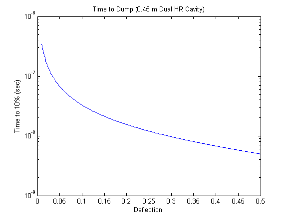
We thus need something that can observe a signal that short.
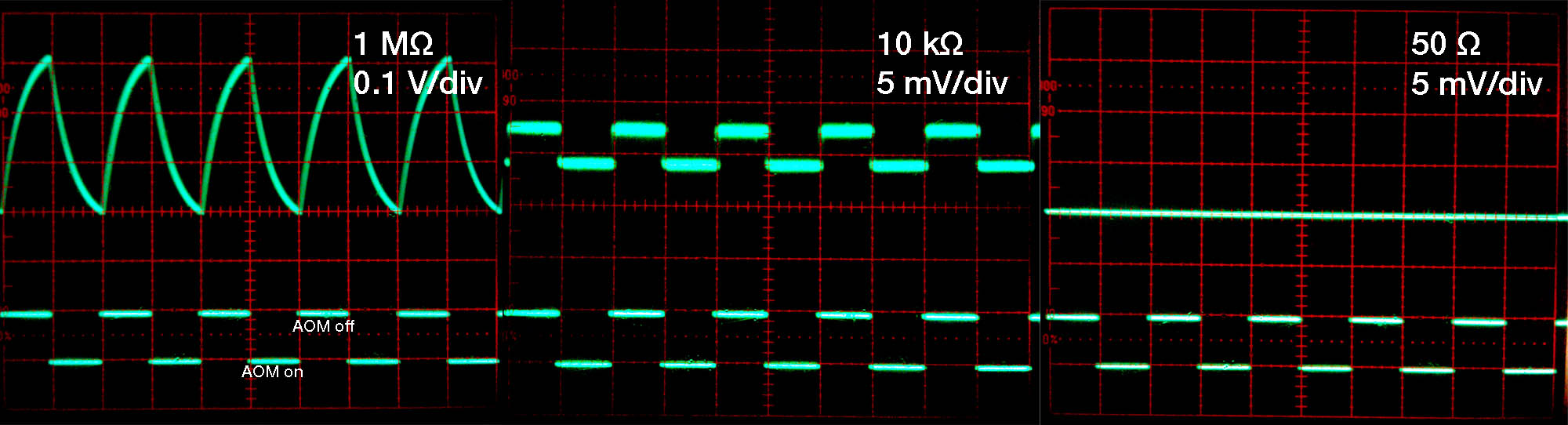
With the oscilloscope set to a 1 MΩ for the resistor, there was a strong, clear signal. However, our time resolution at this resistivity is limited by the electronics. That is, those curves don't actually represent the intracavity light. The time constant for an RC circuit is given by τ = RC. Thus, for high resistances, we cannot distinguish the actual cavity characteristics from the effect of the time constant.
Why not just decrease the resistance? We want to, but unfortunately, resistance is also related to the output voltage of the photodetector. The output voltage (according to the manual) is given by Vo = 0.4P * R. Our power is already very low, and decreasing resistance from 1 MΩ to 10 kΩ resulted in a signal that was too low to reasonably measure (and the time constant might still be too high). Setting the oscilloscope to the highest sensitivity yielded only about 5 mV of signal, not enough to examine the characteristics of the cavity. Going down to 50 Ω resulted in an immeasurably low signal. The photodetector we have is not sensitive enough for the job.
We did, however, find another model, the PDA10A, an amplified silicon photodetector, which might just do the job: It's fast enough, and works well at 632.8 nm. We ordered one, and it should be here tomorrow.
Update 7/30/2013: I found the amplifier in the lab today, but the neither the amplification nor the noise level were satisfactory for use.
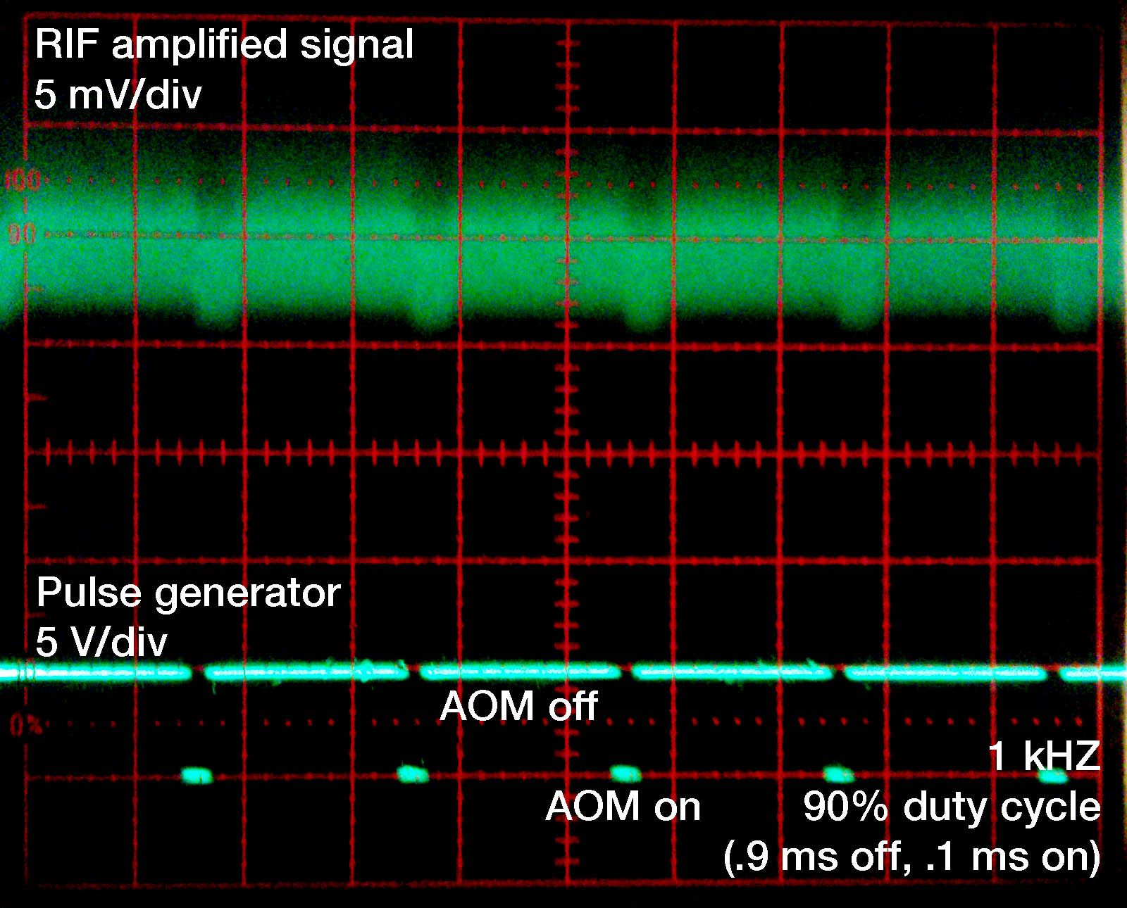
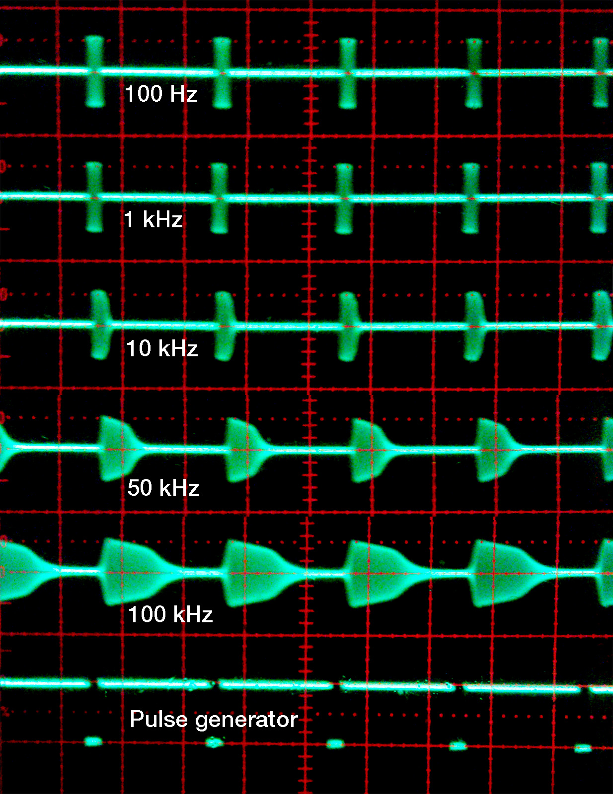
The duty cycle of the pulse generator was set to 90%, and I looked at various pulse frequencies ranging from 100 Hz to 100,000 kHz.
We can see that the pulse quality deteriorates past about 10 kHz. Square VHF pulses become temporally longer and unsquare as we increase pulse frequency. By 100 kHz, the duty cycle looks nothing like 90%, and the shape is quite round.
On Friday and Saturday, I set up the pulse generator with the VHF oscillator in attempt to cavity dump the laser. I removed the AOM from the cavity for a while to test it out with a regular beam of light. I found that there was significant deflection at 25 MHz, though the beam appeared to be under half deflected, even at full power (that is, much of the light still went straight through).
I took a while to read the instruction manual of the pulse generator before connecting it to the VHF oscillator. After playing around for a while, I ended up selecting 5.5 kHz, .1 ms width pulses to feed the oscillator. A lens focused the waste beam of the HR onto a photodiode.
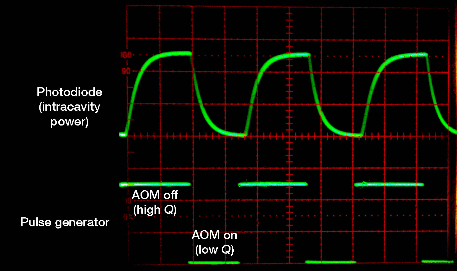
My original interpretation of these readings:
The AOM is turned off, enabling the laser to resonate and build up intracavity power. This is shown by the photodiode trace curving up. The AOM is turned on, deflecting part of the beam out of the cavity. The laser stops resonating, and the circulating power is ejected from the cavity after several round trips (accouting for the gradual fall). The laser is successfully cavity dumped.
I was suspicious though: It should not take 100 μs for all the light to be ejected from the cavity. A 100 μs ejection time equates to about 40,000 roundtrips in the cavity, which doesn't seem right. I discussed this with Dr. Noé, and he said it was probably due to the RC time constant. That is, the rise and fall time of the system is not limited by the photodiode, but rather the electronics between the photodiode and oscilloscope. The slope was due to the gradual charge/discharge of the capacitor, NOT an actual photodiode reading. This was confirmed by inserting a resistor with different resisitivity inside the circuit. The photodiode trace looked different. I will have to discuss with Dr. Noé and Marty tomorrow to determine what I should do next.
An estimation problem with lasers:
|
Given a red HeNe with a Fabry perot cavity the length of Long Island, (1) What is the frequency spacing between two adjacent longitudinal modes in the cavity? (2) How many lasing modes would be present at a given time? |
A laser resonator contains many standing waves which are resonating. The frequency (mode) spacing is given by:
A quick look at Google Maps shows that Long Island is about 200 km long.
The gain bandwidth (fwhm) of helium neon is 1.5 GHz.
Yesterday was the weekly pizza meeting. Giovanni (PhD candidate at the City College of New York) came to visit with Stefan and gave a talk on optical vortices, classical entanglement, and its applications in telecommunications. Because the spatial and polarization properties of these vector vortices are independent of each other, more channels can be sent down a fiber line. It was really interesting to follow along the cutting edge of the science behind telecommunications: This will definitely be huge in a few years.
We also toured the ultracold lab down the hall in the physics basement. It was the first time I had been in a Bose-Einstein condensate lab, and the complexity of it was pretty impressive. They have a bunch of laser systems, and it'll be interesting to look into BECs, a topic I'm not very familiar with.
Sam's care package also came recently. The contents include a bunch of AOMs, the second 45 mm HR that I was so desperately looking for, some useful cables, and the feedback circuit for the stabilized HeNe.
Because we want an AOM with minimal loss (to place it inside the cavity), I tested a few of them with a power meter to see which one reflected the least amount of 632.8 nm light. The one designed/coated for 632.8 was (unsurprisingly) the least reflective. The reflectivity was unmeasurable on the 1 mW scale. Additionally, that AOM has a large opening to the optical medium, which makes alignment a bit easier. Mounting it to any platform was a challenge, as it was an irregular height with irregular screw holes.
Marty found a VHF generator and showed me how to use it. I hooked it up to an oscilloscope, and found that it was calibrated fairly well, but I found that its power might not be enough. We played around with the a few of the AOMs outside the cavity for a while. One of the AOMs operated in the Bragg regime, producing only a single diffracted beam (or possibly two; one on either side, depending on the angle). The other operated in the Raman-Nath regime, producing several orders of diffracted beams.
We found that the AOM we selected for intracavity operation operates primarily in the Raman-Nath regime, which isn't favorable for cavity dumping (we want a single dumped beam, not multiple orders), but the angle of incidence can be adjusted to produce just a single diffracted order.
Another problem was that the AOM does not deflect the beam much. To view the higher order diffracted beams about 2 centimeters apart, I had to let the beams diverge for about 3 meters. This isn't a good thing when our cavity is only 45 cm long. Marty suggested that we could look at the HR waste beam to analyze what's going on inside the cavity (without actually seeing the dumped beam exit the cavity). I think that some clever mirror placement might allow us to view the dumped beam though.
I made a mount which places the AOM inside the cavity. It seems pretty sturdy, and the laser continues to lase well with the AOM inside. I'll be studying what happens when I turn on the AOM tomorrow. It might also be a good idea to characterize the AOM and investigate its properties. Pictures of everything to come.
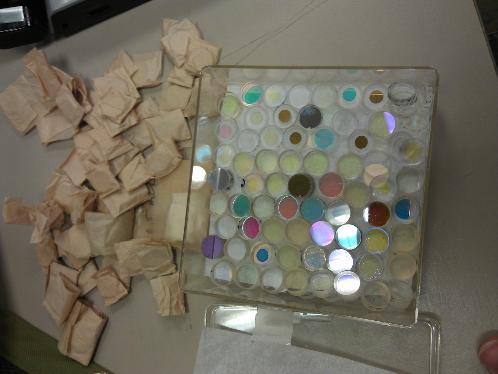
I found a big box of laser mirrors (there are at least 200 mirrors) in the lab today. Neither Dr. Noé or Marty know where it came from. All of them are labeled with pencil on the sides, some clearly, some not so clearly. There are mirrors of all different coatings and thickness, but most of them seemed to have a 2 m focal length. Some of them were in good condition, some quite damaged.
Marty took a look at the transverse modes produced by the aperture inside the open cavity laser. Because the beam focuses to somewhere in the middle from either side of the cavity, he suggested I place the aperture near the output coupler to gain some resolution in cleaning the modes. By doing this, the beam width would be larger than at the center (where the aperture was previously), and thus easier to manipulate. When I tried it, the aperture adjustment was slightly less sensitive, but I also was no longer able to adjust the cavity length. Marty also suggested that (while waiting for the modulators from Sam) I investigate and see if there's a relationship between beam diameter and cavity length. I'm reading a bit on resonator design to see if I can get any insight on this.
I found a beamsplitter lying around, so I put together a basic Michelson interferometer today just for fun. You can see the fairly clean TEM00 transverse shape of the beam. Moving the fringes over by one is equal to a mirror movement of λ/2, or 316.4 nm, roughly two orders of magnitude smaller than the diameter of a human hair.
Here's another estimation problem:
I remember reading from Sam's Laser FAQ that the maximum intensity of sunlight at ground level is approximately 1 kW/m2. Using Google Maps, I estimate that about 20% of the Stony Brook campus (total area) is covered by roofs. Also using Google Maps, I estimate that the Stony Brook campus (relevant to our estimation) is about 2.5 km2. Using dimensional analysis,
we find that about 2.5*106 kW of power reaches the rooftops of the campus buildings at any given moment. Solar cells vary in conversion efficiency. Thin film photovoltaics might be about 10% efficient, while high end silicon photovoltaics might reach over 30%. Using a conversion efficiency of 20%, we find that the output of the solar cells is about 5*105 kW. In 12 hours, we can generate 6*106 kWh of energy.
6*106 kWh of energy is enough to keep 6,000 average American homes operational for a month (1,000 kWh per home per month).
There are 3.6 MJ in 1 kWh, so 6*106 kWh ≈ 2*107 MJ.
I elevated and mounted the open cavity adjustable HeNe to the table today. It was kind of difficult because the laser was mounted on wood, which isn't a very stable surface. I tied a few lab jacks to the table, then placed the laser assembly on top of them. Using long mounting posts, I put braces in three positions of the wood base. The resulting assembly looked pretty nice, and was definitely stable. Adjusting the height of the laser, if needed, won't be difficult.
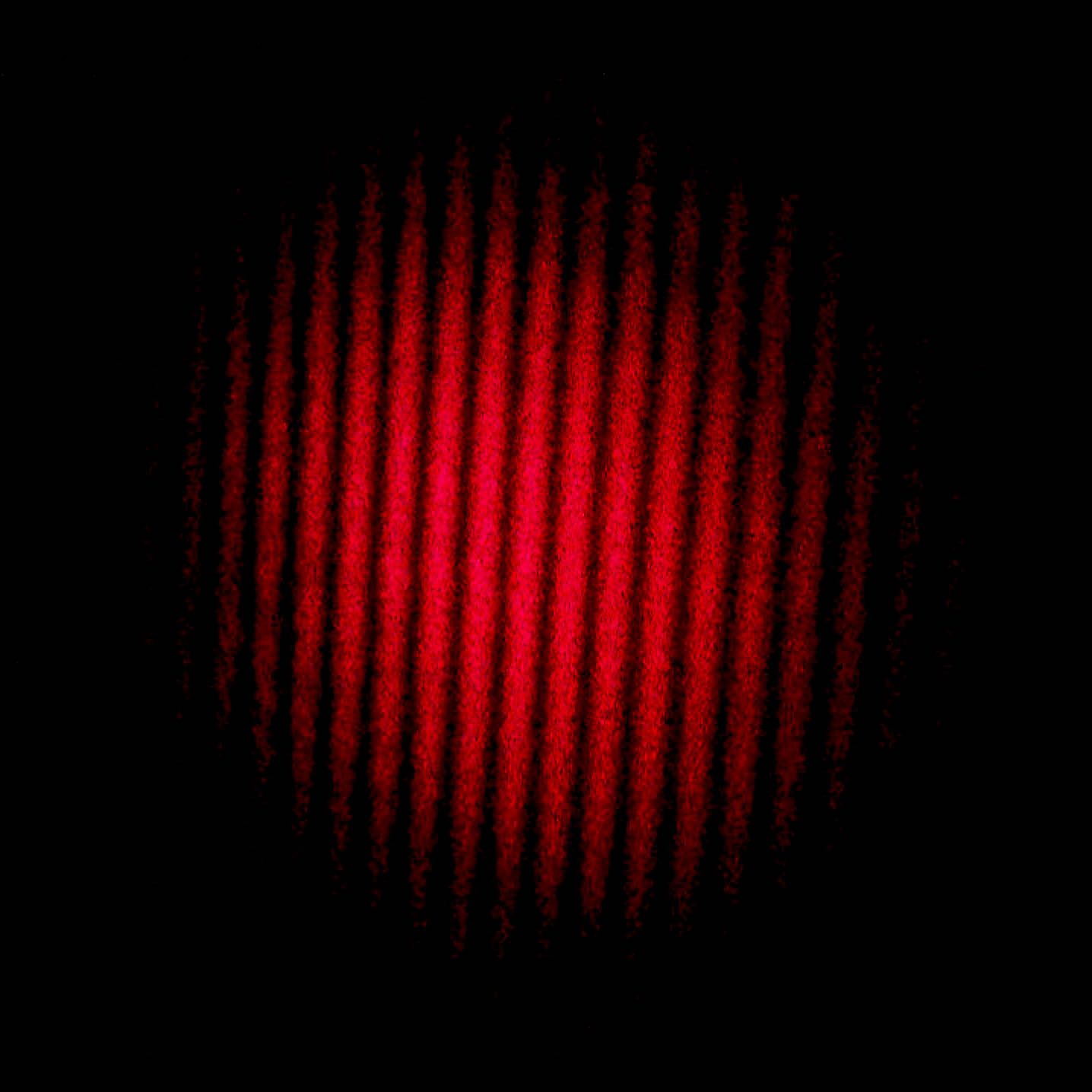
The open cavity laser produces very high order transverse modes. When expanded with a lens, it's apparent that the modes are very complex. To clean them up, I mounted an iris to a 3 axis micrometer stage, then closed it down. I was able to clean it to a TEM00 beam with the aperture.
I spent the morning preparing for my talk about ultrafast spectroscopy, which I had already given during my first Wednesday pizza talk. Because Sam was here, I foucused more on the laser aspect of my talk. I also added some more information on modelocking, and gave a quick introduction to basic time and frequency descriptions of how it produces pulses of light.
Sam also taught us about basic laser operation during the talks. He gave a great overview of all the different categories and specific types of lasers, which was quite informative. His discussion on laser operation would definitely have helped those without a laser technology background understand how they work. After he talked about Fabry Perot interferometers, Hal brought up confocal mirror assemblies and explained how their FSR is c/4L rather than c/2L.
The others also gave talks and gave a quick progress report on what they've been doing lately.
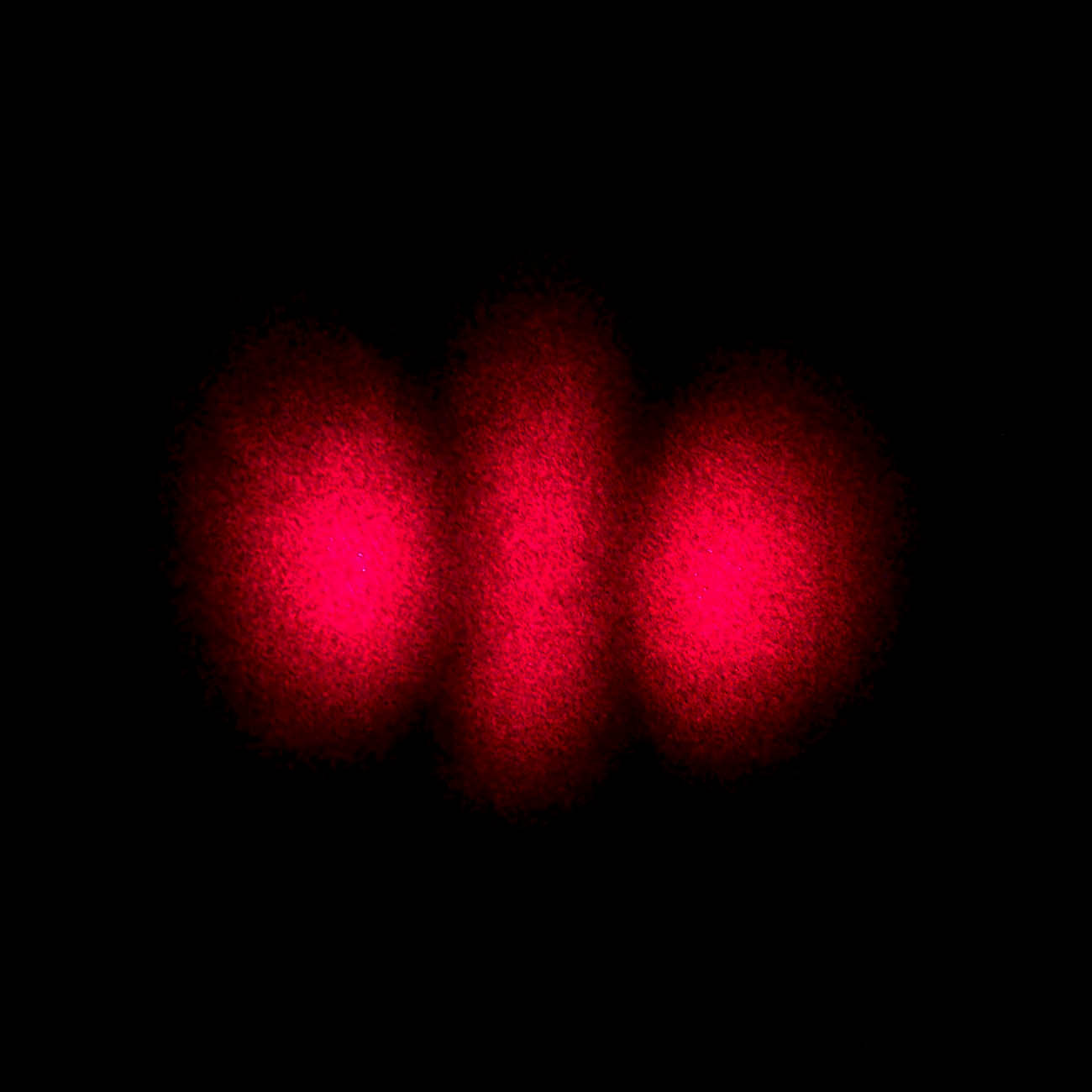
I played around with the (relatively) fixed cavity length open cavity HeNe today. Adjusting the OC mount, I made some nice modes. Here's a TEM02 mode:
Marty thought of some things to do with the open cavity rail adjustable HeNe that Sam brought in. This particular HeNe tube's gain is a bit stronger than other tubes: It continues to lase even with the addition of a glass microscope slide near the Brewster's angle inside the cavity. Intracavity modelocking might not be too practical (the AOMs we have are too lossy), but Marty suggested replacing the OC with another HR mirror and inserting an AOM or EOM to cavity dump the laser. The way the cavity recovers after each cavity dump can be analyzed to give information about the HeNe tube.
Also, this laser produces many higher order transverse modes. It'd be interesting to manipulate them (using intracavity apertures/pinholes) and observe them. I'm currently working on mounting the laser to the table and getting something set up for that.
Dr Noé took everyone in the group (including Sam, Hal, and Dave) out to dinner. We didn't talk too much about optics, but it was nice to see everyone outside the lab. The food was good too.
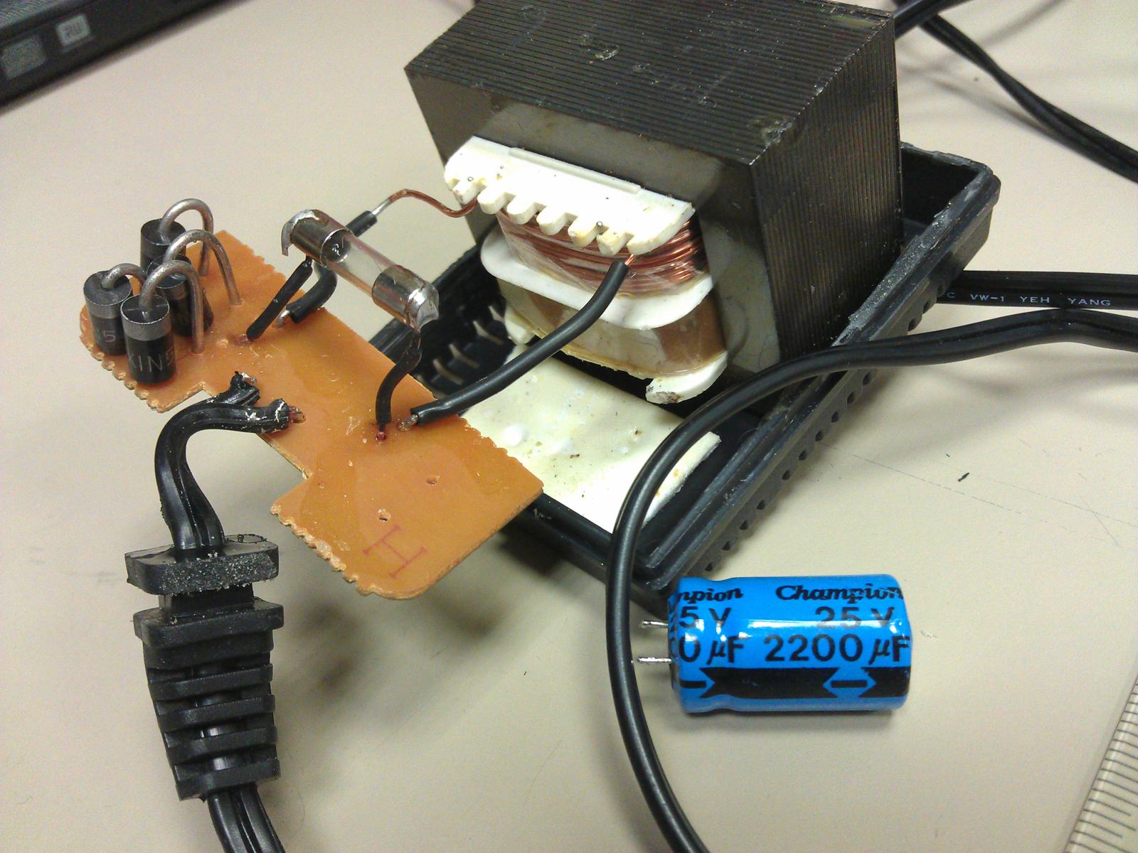
The barcode scanner HeNe that Casey is setting up needs a 12 V DC source at at least 1 amp. I found three power bricks in the drawer rated for 12 V at 1.3 amps, but all three seemed to be dead when tested with a voltmeter. I took the cover off one of them to investigate. Upon inspection, I found that the original fuse had blown. Someone had attached another fuse on top of that, which was also blown. I cut both off and, with the help of Sam, sodered another fuse on. When plugged back in, the fuse blew immediately. The transformer was fine though, but upon further investigation, we found that the capicitor was dead. Unable to find a similar one (and coming to the realization that we were spending a long time on a $10 power brick), we called it quits. I had found another power supply anyway.
Dr. Noé was kind enough to take me, Casey, and Sam out to dinner today. We had some nice discussion over dinner. Some topics we talked about/I'll be thinking about include:
Laser Sam came today! After a lunch at the Simons Center, he helped me and Casey fix up a frequency stabilized, single mode HeNe. The total cavity length was about 25 cm. We soldered the laser power supply to the ends of the tube, then redid the insulation around the HeNe tube. After hooking it up to a power supply, it functioned as expected!
We found a nice jack to elevate it to the height of some mirrors we placed, then focused the beam through a Fabry Perot interferometer. We observed the laser's longitudinal modes with a high speed photodiode on the other end of the interferometer.
Because the cavity length of this laser is so short (making mode spacing, c/2L, large), only two modes (or maybe a third tiny one) can fit under the gain curve of the neon gain medium. Both of these modes are polarized perpendicularly relative to each other, so we used a linear polarizer to selectively filter out one mode. The result is a frequency stabilized, single-mode HeNe laser.
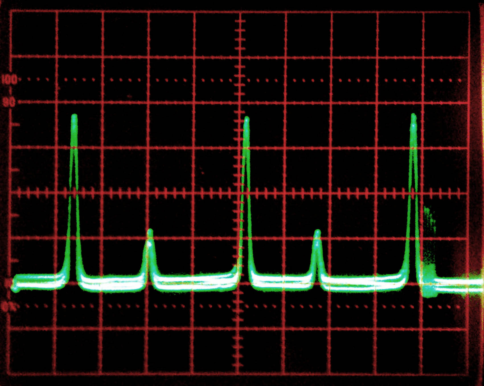
Here, you can clearly see the two modes of the laser: One is the tall peak, and the other is the short peak. The horizontal axis represents wavelength (it's actually time: the Fabry Perot scans wavelengths over time, so it essentially represents wavelength), and the vertical axis represents intensity. The two peaks repeat themselves three times in the picture because the Fabry Perot cycles three times in one scan of the oscilloscope. The distance between the two peaks (the tall one and the short one) represents mode spacing (also known as axial spacing or free spectral range, FSR), which corresponds to c/2L.
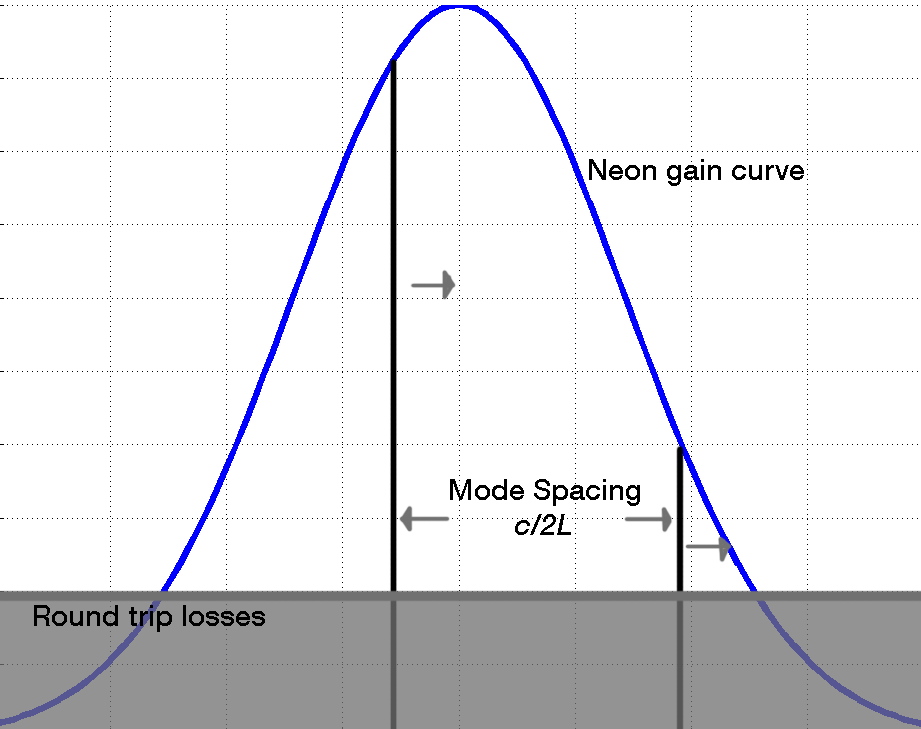
The reason why one peak is taller than the other is apparent upon examination of the mode diagram. Lasing occurs when gain exceeds losses, but only discrete modes (those standing waves that constructively interfere) are allowed in the cavity. In our laser, two modes (vertical black lines) fit under the gain curve. Unless those modes happen to be the same distance from the center of the gain curve, they'll be different in intensity.
As the laser heated up after turning it on, the cavity expanded. As such, the supported modes swept to the right, and you could clearly see the to mode peaks on the oscilloscope sweeping to the right and changing in height, as well as new modes appearing from the left.
We placed a linear polarizer in front of the Fabry Perot. Because the modes are polarized perpendicularly relative to each other, rotating the polarizer selectively filters one mode or another. When the polarizer is 45 degrees relative to both modes, both modes are let through equally (as shown in the oscilloscope above).
We went over the estimation problem from a few days ago:
I considered the Airy disks created by the iris of the human eye. I was interested in the diameter of the first maximum, as two points project on the eye would have to be separated by at least the diameter of an Airy disk to be distinct. Using the equation for Airy disks,
for small angles,
Using λ = 420 nm (the average of visible wavelengths) and d = 6 mm (an estimation of pupil diameter), I calculated θ ≈ 9 * 10-5 radians. All of us were pretty close with our results, on around the 10-5 order of magnitude.
Samantha also talked about the Python programming language, which (with the right packages) can come in handy for generating graphs. We browsed the American Journal of Physics for a while after that. All of us encountered articles that had interesting titles, and I'll be skimming them over the weekend.
An interesting topic that I read about was the solar pumped laser. Rather than using electricity as the pump source (as most all lasers do), these lasers use the sun as a pump source. They're much more efficient than any regular laser. Solar pumped lasers could have interesting applications in space and magnesium power sources (due to their 'easily' attainable high cw power outputs). Current research on solar pumped lasers seem to be focusing on improved efficiency and higher power, so I'm not too sure what I might be able to do with it. I'll be thinking about it though!
At the pizza lunch today, we all met Samantha and learned a bit about her work in astronomy. Her talk was really informative: Astronomy is not something I know much about, but she explained the basics clearly for us. Her work with blue stars and the SDSS seems like a really gargantuan task, and very helpful for the scientific community. After eating the pizza and a LTC group meeting, Dr. Noé showed us a few antique books he bought while he was away.
During the group meeting, I talked about my interest in laser technology modelocking a HeNe laser. I think I'd be really interested in a project involving that. Another interesting idea brought up was creating sound beats with two lasers very close in frequency and a loudspeaker. Kathy also discussed how a beam interacts with a dichroic mirror differently depending on the side the beam is incident on. It was brought up several times that Sam Goldwasser ('Laser Sam') from Sam's Laser FAQ will be around the LTC next week. I'm really excited to meet him ‒ his exhaustive and comprehensive resources on laser technology have really helped me out over the past two weeks.
I've been learning more about the workings of a laser lately. I've also started reading into Gaussian optics, as it seems like a good place to start. Because Fourier transformations have come up quite a bit in my reading, I've been learning about Fourier series and expansions as well.
A few of us left the lab a bit earlier than usual today to go tour the Allison Group's lab. I asked Melanie Roberts, a postdoc in the newly-formed group, if she could show us around. She gladly let us in for a while to talk about the group and their work. Their setup has components that do the same thing as a traditional ultrafast lab (ti:sapph), but individual components are different. The group uses fiber, as opposed to titanium sapphire, as a gain medium for their modelocked laser. I haven't read much about fiber lasers, but Melanie explained how they were much more stable. So stable (and compact) in fact, that they were able to make the move from the physics to chemistry building without having to rebuild the laser, as the entire assembly was mounted on a breadboard. The modelock is not easily lost either, so they don't have to worry about bumping the table and losing the mode. Because they're just getting started, they just have this laser and an autocorrelator built so far. If I'm ever around Stony Brook in the future, I'll have to be sure to stop by again!
We profiled the TEM00 beam from a Keplerian beam expander today.

A 5 mW HeNe laser beam was sent through a simple Keplerian beam expander made of two plano-convex lenses. The focal length of the first lens, f1, was 0.125 meters, and the focal length of the second lens, f2, was 0.750 meters. They were aligned such that their focal points were at the same position (that is, distance = f1 + f2). The magnification factor of the system is f2 / f1 = 6.
A photodiode with an aperture of 200 microns was placed on a stage under 0.5 m past the second lens and was moved in 100 micron (0.1 mm) increments from one side to another along the vertical center of the beam. We started collecting intensity readings well before the beam began picking up in intensity.
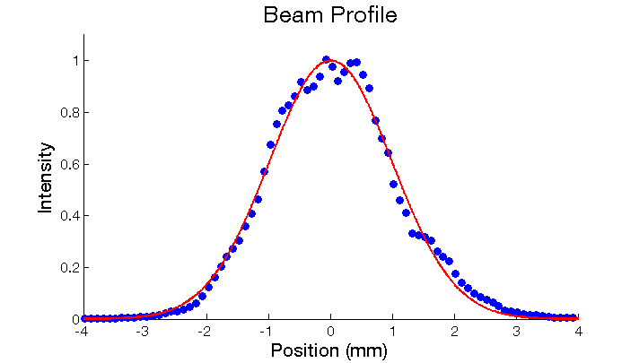
The intensity vs position values shown above were scaled to arbitrary units, and translated such that the position of the maximum is 0 mm. The blue dots represent our collected data, and the red line is a least-squares Gaussian fit. The calculated 1/e2 diameter of the beam is 3.99 mm.
The beam was collimated well, maintaining its size immediately out of the second lens to over 25 meters away. At all of these distances, the beam looked like what it's supposed to, with no noticable point bright or dark spots. At very far distances (>10 m), the messiness around the main beam was gone, probably due to divergence. The lenses, though not cleaned before usage, did not seem extremely dirty. What would explain the messy peak and the shoulder at about p = 1.5 mm?
Because we couldn't find a stage for the photodiode that was both tall enough and had the right screw size, we placed one stage on top of another as an extender. Unfortunately, the bottom stage had a loose connection somewhere, and as such, was not completely tight. Although we were careful not to wobble it, it is absolutely possible that accidental shifts accounted for movements of over 100 microns, perhaps causing the shoulder on the curve and the messiness of the peak.
We learned a bit about setting up optics on the table. It's actualy quite a tedious process to align everything perfectly ‒ it took us a while to find the right stages, mounts, and screws.
I also did the estimation problem from a few days ago. My work is here.
We went over the tire estimation problem today. Surprisingly, we were all within an order of magnitude of each other. Even more surprisingly, Kathy and I estimated the same exact number! Melia gave us another estimation problem today:
|
Given an aperture the size of the umbilic torus and a red HeNe laser, (1) What focal length lenses would be needed to fill the aperture? (2) At least how far would we have to be to see the far field diffraction pattern? |
I spent most of my day typing up some of my notes from the laser book I was reading. Some of my notes on birefringence can be found here
Melia showed us an estimation problem this morning. I have had some experience with them already in Science Olympiad. The idea is simple: Break the problem down to make the assumptions as easy as possible, then use dimensional analysis to work for what you're looking for.
To begin,
Using dimensional analysis:
Continuing,
Consider the .25 cm outer worn portion of the tire:
Some final dimensional analysis:
I continued to expand my knowledge about lasers. Rather than jumping around the internet with my reading, I decided to read some more format writing about lasers. So before I continue reading the thesis on modelocking, I made my way through the first ten chapters of Hitz, Ewing, and Hecht's Introduction to Laser Technology. They give relatively elemtary, yet detailed explanations of light and lasers. Although I was familiar with much of the content, it did help clarify some of the details I was stuck up on. Also, it helped explain some concepts with less mathematical rigor, which helped me understand them more clearly.
I found an undergraduate thesis by Sam Spencer, a student from Reed College, on the modelocking of a HeNe laser. I'm still reading through the first chapter about basic laser operation and modelocking theory - Spencer explains quite well. I also found Ewuin Guatemala's LTC page, and read about his work with HeNe modelocking. During a brief disucssion with Marty about the thesis and his experiences with Ewuin, he revealed that the two cases were almost identical. Marty also said that Ewuin's progress was halted by the end of the term, so many unanswered questions remain - this could be an interesting area to investigate.
From what I have read so far, it appears that both Spencer and Guatemala actively modelocked the laser using frequency modulation with acoustooptic modulators. I have yet to read further about the actual experimental design, but I'm looking forward to seeing how it was done. I'm also still familarizing myself with some of the terminology and phenomena behind modelocking.
On Friday, Dr. Noé walked us through an approximation of the interference pattern created by double slit diffraction.
To begin, we start with a representation of plane waves in complex notation:
where
k is called the wave number. A spherical wave can be represented by the same equation multiplied by \frac{1}{r}.
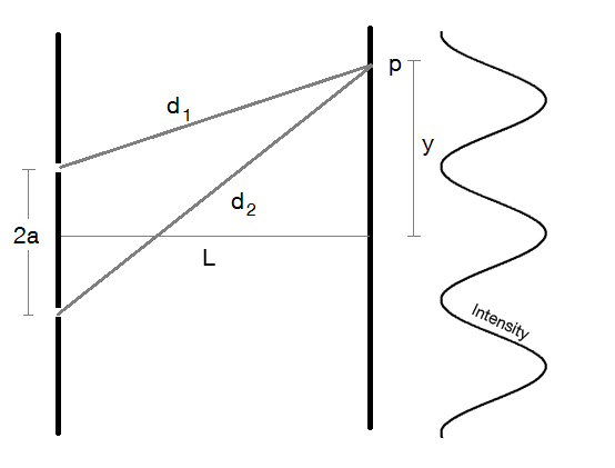
Plane waves hit a wall with two slits separated by distance 2a. A parallel screen is distance L away from this wall. Point p is distance y away from the middle of the two slits d1 away from the upper slit and d2 away from the lower slit (see diagram below).
We are not concerned about time or the decrease in intensity over distance (because we are working in the far field, that is, with large L. The amplitude at point p, Ap, is:
The intensity at point p is
where A'p is the complex conjugate of Ap.
Substituting,
After some manipulation with Euler's formula and the binomial expansion theorem (eliminating all complex terms and rewriting d1 and d2 in terms of L and y), we arrive at:
This is an approximation between intensity and position along the second wall for sufficiently large L.
We also went over small angle approximation, which can be useful for estimating laser divergence.
I spent the day looking in to some interesting topics in optics. My next order of business will be to consolidate my ideas (currently on paper) into an ideas page - that's my plan for tomorrow. I've been investigating the working of lasers and methods of producing pulsed laser light. A few methods I've looked in to are modelocking, Q-switching, and cavity dumping. Analyzing pulse shaping techniques might be interesting as well. I'm quite in to photography, so I read about moire/aliasing patterns, and I also read about some very introductory lens design. I find video in the anamorphic format to be very cinematic-looking and aesthetically pleasing. Producing true anamorphic format video requires lenses that are expensive and thus impractical to the average student video/film producer (like me). An interesting investigation might be to see how one can produce an anamorphic-looking video without the expensive equipment.
We also had a workshop on lab safety today, but it was essentially all about wet lab procedures, therefore largely irrelevant to anything in the Laser Teaching Center.
I gave a short talk on my experiences at the University of Minnesota today. Since January this year, I've been working in Professor David Blank's ultrafast spectroscopy lab. Over the past few days, I have been reviewing some of the optical systems on their laser tables. Today, I talked about the basics of pump-probe spectroscopy, and some of the fundamental optical systems that it needs to operate. A mode locked titanium-sapphire oscillator provides the gain medium for the laser and ultimately outputs an 85 mHZ pulse train that is sent to a regenerative chirped pulse amplifer. The end result is a clean, 1 KHz, 60 fs, 400 μJ, 810 nm pulse train usable for pump probe spectroscopy. Another system is the noncollinear optical parametric amplifer, which takes in the 810 nm pulse train from the regen and tunably turns it into any wavelength from about 450 nm to 700 nm.
The other talks today were also interesting. In particular, Casey's talk on his studies of HeNe lasers helped clear up some of the confusion that I have been having with understanding the workings of the TiSaph oscillator. I'm sure that his research page will certainly prove useful in the future.
Dr. Noé mentioned today that someone had a pico projector. Of note is the fact that it contains a native green (≈530 nm) laser diode. Almost all green lasers today are actually natively a 1064 nm infrared laser with a nonlinear frequency doubling crystal. This laser natively outputs green light without any need for a doubler, which should be more efficient and make the beam more stable. I found an publication (Appl. Phys. Express 2010, 3, 61003.) that had references (specifically #2-10) to many other publications about native green lasers, which should be some interesting and challenging reads.
The Simons program began today. After an introductory breakfast, the two other Simons fellows and I went to the Laser Teaching Center with Dr. Noé to take a tour and do some demos. There, Noé showed us some interesting optical phenomena. The interferometer, constructed from a beam splitter and a few mirrors, allows tiny distance measurements to be taken. It works by the same principle as beats produced from two slightly detuned audio tones. Placing materials with long chained molecules between two linear polarizers causes them to appear to turn different colors. Rotating the polarizers causes a color change, but rotating the material may or may not change the color (depending on whether or not the molecules' chains are randomly aligned).
After lunch, we had a group discussion about the talks we'll be giving on Wednesday. Noé explained the importance of crafting titles: A strong title will get the attention of audience members and not be overly specific. We also had a discussion about what we'd be talking about. I will be presenting the project I worked on in Professor Blank's ultrafast spectroscopy lab at the University of Minnesota, and also talk about some optical systems we used on his laser tables. Afterwards, I talked with Rachel about some of my interests in optics, and came up with some possible areas of investigation. Noé also posed a question: How could one find the orientation of a linear polarizer without a polarizer with a known orientation? You'd need a source of polarized light with a known orientation. After some reading, I discovered that light reflected at the Brewster's angle off non-metallic surfaces is all s-polarized (perpendicular to the plane of incidence). Therefore, when you turn a linear polarizer such that it blocks all the reflected light off a non-metallic surface, you know that it's vertically oriented.