Experiments with a Consumer Digital
Camera in the Optics Laboratory

I. Introduction / Goal

II. Experimental Tools

III. Experiment Setup

IV. Measurements & Analysis

V. Conclusions

VI. Acknowledgements

VII. Further Reading

I. Introduction

By its nature, a digital device segments raw data into distinct datums. However, that is not the only change that such devices make in interpreting information. Colors are sometimes altered, as are intensity levels, to form a more pleasing photograph. While this is an acceptable practice for creating art, it is not for accurately recording information. A plan is needed to find out how exactly a digital camera operates in general, to explore the specific changes made by the digital camera at the lab, and to determine how to minimize such problems.

The overall goal of my project was to test the usefulness of a standard consumer-type digital camera in an optics laboratory. For example, Mirna Lerotic and Jose Mawyin have collaborated on a project in which interference patterns produced by laser light were recorded in such a camera and later analyzed to determine the "visibility" (contrast ratio) of the fringes. Their analysis is only valid if the intensity values obtained are accurately proportional to the actual light levels in the pattern. I hoped to study this question by studying patterns with known intensity variations.

In my initial research, I tried to get a general evaluation of the usefulness of the digital camera through the web and the creation of simple experiments. The experiments I created involved taking photographs of diffraction patterns and comparing the intensity levels in the pictures to Fraunhofer's and Fresnel's diffraction patterns and other models for the behavior of light. A similar process was used when analyzing the effect the camera has on colors. Through these processes, I planned to discover the severity of the problems inherent in using a digital camera to record information, and what solutions, if any, are available to improve the reliability of the medium.

After some preliminary experiments it became clear that the camera does in fact distort intensity levels in complicated ways that probably couldn't easily be understood in a few weeks. For example, I took a color photograph of a red gaussian band from an uncollimated (unfocused) diode laser. I found that although the beam is actually a uniform frequency, or color, in the photograph the areas with greater intensity, specifically the center, appeared yellow. Further evidence of distortion was shown by graphing the intensity of the gaussian band. The central bell of the gaussian curve was compressed, and the base intensity was raised well above zero.

In view of these complications, the focus of the current project was re-directed at a more specific and hopefully easier question: can one obtain accurate position information about light patterns from such a camera? The initial question about obtaining valid intensity information is being pursued in longer-term projects by Jose and others.

top of page

II. Apparatus and Experimental Tools

The most important apparatus I used was the Sony Mavica digital camera, model FD-73. It saves pictures on floppy disks as 640x480 pixel .jpg (compressed) files. The camera has a 10x optical zoom feature that allows good magnification at far distances. When the zoom is minimized the camera could take pictures as close as one cm away from the lens, at which distance the field of view was about 2 cm.

I also used a standard low-power He-Ne laser made by Metrologic. Its red beam has a wavelength of 632.8 nm (one nanometer = 10^-9). Want to know more? Detailed specifications for the camera and laser are here.

The "experimental tools" consisted mainly of the software programs used to analyze the data, make figures and write this html report. Except for the DOS spreadsheet QuattroPro, these programs run in the linux operating system environment used in the Laser Teaching Center. I also used a dial caliper to measure the diameter of the screwdriver (see next section) and a tape measure to measure longer distances.

• There are many good references to linux and unix on the web. For example NACSE.ORG has a A Scientist's and Engineer's Guide to Workstations and Supercomputers and Prof. Fitzpatrick at The University of Texas at Austin has a Introduction to Computational Physics that includes an overview of linux and linux commands.

• The unix translate command was used to convert the data file from multiple-value lines to one value per line format.

• Emacs is the powerful unix/linux text editor. It was used to reformat picture files and to write this html document. Reference cards of Emacs commands are available from many university sites: try Stanford for an html version and Colby for a printable postscript (.ps) format.

• HTML or hypertext markup language is the programming language of the internet used to create web pages. One can view the html code of any web page by selecting "view source" from the browser program's menu. The main reference used was the book "HTML for Dummies: Quick Reference, 2nd Edition" by Deborah and Eric Ray.

• QuattroPro (QPro) is a DOS spreadsheet program. Although it is no longer used much it is still very useful and efficient. (The whole program fits on one floppy disk.) QPro was used to analyze the numerical data file created from the photograph and to plot graphs. Data and graphs are transferred between the DOS and linux machines by "sneaker-net."

• XFIG is a freely-available vector drawing program. It was used to create the pictures (drawings and formulas) in this report.

• GNUplot is another standard freely-available unix/linux program. It was used to make intensity plots from reformatted pixel arrays obtained from the pictures, and to plot theoretical diffraction patterns.

• XV is an image manipulation program. It was used to examine, modify and convert the .jpg photographs from the camera. It was also used to convert the .eps (postscript) graph file from the QPro spreadsheet into a .gif form for use in this report.

• Last but not least, the powerful search engine Google was used to search for all this information on the web! Google is based on a linux "server farm" with more than 8,000 individual computers.

III. Experimental Setup

The interference pattern that was studied is a type of "two-slit" pattern. It was created using common laboratory objects (a screwdriver and a drill gauge) whose dimensions were either accurately known or could be accurately measured. Because the hole in the drill gauge is round, not square, the two "slits" are actually shaped like tall and narrow crescents, as shown in the following figure. The diameter of the screwdriver was measured with a dial caliper to be 0.120 inches (3.048 mm). The #28 hole in the drill gauge was 0.140 inches (3.556 mm). This makes the maximum width of each crescent 0.010 inches (0.254 mm).

This is a picture of the slits formed by the
screwdriver and drill gauge (drawn to scale).

In order to create the interference pattern laser light is shined on the screwdriver-hole unit and the light passing through the two slits is viewed on a distant screen. The laser was placed 205 inches (about 17 feet) back from the slit unit so that the laser beam diameter would have a chance to expand from its original 1 mm diameter to about 9 mm, or 1/3 inch. A large distance to the screen is needed for two reasons: for one thing the pattern does not assume its final or "Fraunhofer" form for a certain distance, in this case a few feet. Secondly, distance is needed to allow the pattern to expand to a size that can be conveniently photographed. The spacing of the pattern (which consists of a series of equally spaced bands) can be estimated from Young's formula:

Young's equation

From this formula the angle between two successive bands in the pattern is given by x/L = lambda/d, which has the value 0.21 milliradians. (One milliradian corresponds to one mm divergence per meter of path.) This divergence is actually quite a bit smaller than the divergence of the original laser beam, which is 1.7 milliradians.

The resulting diffraction pattern was projected onto a piece of graph paper, which acts as a semi-translucent screen. This is a novel feature of the set-up: the arrangement allowed me to photograph the pattern from behind at no angle, thereby eliminating any parallax that might occur if the photograph was taken from the laser side of the paper, at an angle.

The L was measured to be 235 inches, or 5.97 meters. However, there was a larger than normal error in this value of 10 inches, or 0.25 m. This was because the precise location of the graph paper was not measured immediately, but rather marked on an adjacent white board, and the mark was erased before the precise distance was recorded. Fortunately, I remembered the general location of the mark, and was able to approximate its location.

The overall setup is pictured below (not to scale).

IV. Measurements and Analysis

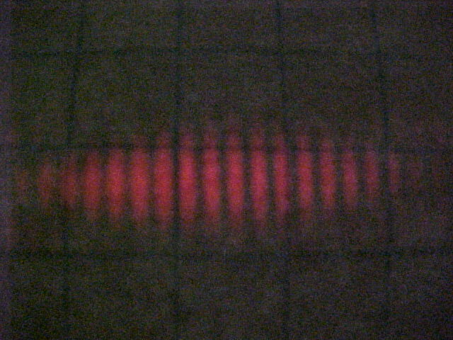
Here is the picture of the diffraction pattern I took with the digital camera. The quadrille pattern on the graph paper that provides the distance scale is clearly visible in silhouette. To see the full size image, click on the image.

diffraction pattern

Next, to graph the intensity, I sharpened the image to create greater contrast between the intensity peaks and valleys. Then I cropped the relevant area, and resized the cropped image to n x 1 pixels. Then I saved the .jpg file as a .pgm (portable-greyscale) file so I would have access to the n pixel values. Within EMACS, I deleted the header and used the translate command (cat file.pgm | tr -s " " "\n" > file.dat) to convert the pixel array from a continuous stream to one value per line. This format was needed for creating the graph in GNUplot (pictured below). In this graph the height of each bar represents the intensity for a given pixel.

intensity graph

The next steps were done in the QuattroPro spreadsheet program after transferring the data file from the linux to the DOS systems on a floppy disk.

The first calculation I made was finding the centroid of the intensity peak for each fringe. Taking the position and intensity from the graph, I found the centroids by using the formula:

Next, I used the centroids' position and peak number to make a linear regression,

the slope of which was the average number of pixels in between adjacent centroids, 33.25 +/- 0.05 pixels. The percentage error in the pixel separation is 0.05 / 33.25, or only about 0.15%

In order to get a separation in physical (distance) units I needed to know a calibration factor relating physical units and pixels. I got this by determining the average pixel separation between two of the vertical graph paper lines, which are separated by exactly 1/4 inch. The technique was to draw a box in the XV program whose left and right sides coincided with the two graph paper lines. The size of this box was then revealed by using the crop and resize commands, without actually resizing. In drawing the box I stayed near the center of the fringe pattern, to avoid systematic errors due to the obvious distortions of the grid lines caused by the paper not being totally flat. I repeated the spacing measurement ten times and calculated the mean and standard deviation of the values in the spreadsheet program. The result was that there are 155 +/- 6 pixels per 0.25 inch, or equivalently, 6.35 mm. Dividing the peak separation in pixels by the calibration factor the result for the peak (fringe) separation in physical units is x = 1.37 +/- 0.05 mm. The uncertainty quoted is given entirely by the percentage uncertainty in the calibration factor, which is 3.9%.

Using Young's formula (d = wavelength*L/x) d was 2.76 +/- 0.16 mm. The percentage uncertainty in d is obtained by combining the percentage uncertainties in x (3.9%) and in L (4.3%) "in quadrature" according to the following formula

Formula for combining errors. The error in
the wavelength lambda is negligible.

This value of d obtained from the interference fringes is slightly smaller than, the measured diameter of the screwdriver, d_screw = 3.05 +/- 0.05 mm. Light that passes closer to an object bends more, so the light closest to the screwdriver was the most responsible for the interference pattern. That is why the diameter of the screwdriver was used for d instead of a weighted average of the diameter of each crescent.

V. Conclusion

Through my study, I have demonstrated that a consumer-type digital camera can be very useful for recording spacial patterns of intensity variation, and I have developed specific procedures that provide an easy means of analyzing the photographs through standard linux programs. The rather large error of almost 6% in the final result for the equivalent slit separation d was determined by the large percentage error in L and variations in the calibration factor caused by the graph paper not being flat. Were the experiment repeated, these errors could easily be reduced greatly. Thus the method seems capable of an overall accuracy of one percent of the fringe spacing, or better. Since the spacing is about one millimeter, the absolute error in such a measurement could be less than ten microns, which is approximately the size of one red blood cell!

top of page

VI. Acknowledgements

I would like to thank both Scarsdale High School and the Laser Teaching Center at SUNY Stony Brook for giving me the opportunity to have such a unique experience. I would like to specifically thank Dr. John Noé, the director of the center, for his help, support, and guidance throughout the past several weeks. I am glad he allowed me to become part of the center's community and to add to its research. I would also like to thank Lisa Bjorndal, the center's teaching assistant, for her personal attention. Her constant pushes kept my mind on task and helped me understand difficult concepts. Also, thanks to my Scarsdale Mentor, Mrs. Jennifer Maxwell. Finally, I would like to thank every one who worked at the lab, or visited, for allowing me to be part of their work.

top of page

VII. Further Reading

1. Hecht, Eugene. Physics: Algebra/Trig. Brooks/Cole Publishing Company, New York 1998. University Press 1998.
2. Hecht, Eugene. Optics. Addison Wesley Longman, Inc. 1998. Inc. 1999. Third Edition.
3. Ray, Deborah S. and Eric J. Ray. HTML for Dummies: Quick Reference. IDG Books Worldwide, New York 1997.
4. My Weblinks.

top of page