Research Journal
August 28, 2014
After a few weeks away from Stony Brook and the LTC, Dr. Noé and I spoke on the phone to discuss progress with my paper. We decided that rather than focusing on new experiments I can do to further my knowledge of and project with birefringent filters, I should instead figure out how to present my work in a paper. We began looking into different applications to incorporate broader themes such as polymers, waveplates, and Jones Calculus. I'll also be working on an informal web report to base my paper off of in the next couple days.
August 12, 2014
Today was the poster symposium! It was really fun presenting to all the people that stopped by. After, Dr. Noé took all of us and our families out for lunch at the Simons Café. I had a great time with Dr. Noé, Libby, Melia, Hal, my parents, Marty, and everyone else. I also talked to Dr. Noé about coming back and using an interferometer to see the fringe patterns generated by my filter samples. We'll also be collaborating in the near future to write a paper.
August 8, 2014
The closer and closer we get to the end of the summer, the shorter and shorter my journal entries seem to get! I spent the entire day today editing my poster. I went through several rounds of edits with Mary, Melia, and Dr. Noé. Hopefully now I'll be able to present an informative, well-made poster.
August 7, 2014
Today I spent the majority of the day finishing up some calculations and graphing the phase shift dependence on wavelength. I also worked on my poster and will hopefully have a draft by this evening.
August 6, 2014
This morning, I prepared my presentation for the pizza lunch in the afternoon. It was just a quick update on the progress I've made since last week. I also talked to Melia about my data from yesterday. With the crossed polarizers, the maxima are indications of horizontal half-wave waveplates, while the minima are vertical half-wave plates. Yesterday I was able to rotate the samples at an angle theta relative to each other to create a horizontal quarter-wave plate, as indicated by the peaks flattening out. Today, I'm going to try to create a vertical quarter-wave plate in attempts to get the minima to flatten out.
In the afternoon, Marty stopped by the lab, and we had a long discussion about my results from yesterday. He and Dr. Noé were a bit skeptical about the graphs since the intensities were so low compared to the previous recordings, so he asked me to do the math again. After modeling everything, I'll be able to tell whether or not what I was seeing was truly polarized light and if one can actually make circularly polarized light at the wavelengths of rotated linearly polarized light (either of which result would be a great scientific finding!).
August 5, 2014
Today was an exciting day! I started off by getting the entire lab Starbucks (Libby texted me everyone's orders)- I have to get rid of my meal points soon!
Once I had my coffee, I set straight to work on building the filter for a QWP. I had to prepare the samples with 2, 4, 6, 8 and 10 strips of parallel tape again so I could cross them with the original samples. In order to make sure I was producing circularly polarized light and not eliptically polarized light, I had to make sure an equal amount of light was passing through the fast and slow axes. I did this by finding the angle at which I must place the sample for extinction and rotating it by 45 degrees. In principle, that should allow the filter to produce circularly polarized light.
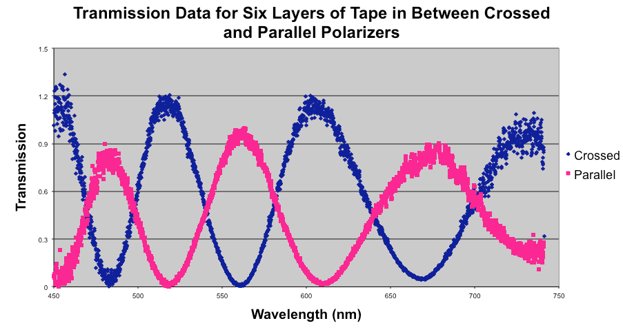
After normalizing my data, I noticed that instead of a flat horizontal line, I was getting a bumpy curve with some broad (but imperfect) maxima. At first I was confused, but upon further discussion with Dr. Noé and Melia, we hypothesized that these forming broad curves could indeed be an indication of a QWP! Looking at crossed polarizers, the maxima for the layer samples are indications of wavelengths at which the tape behaves like a half-wave retarder. Since I'm trying to create a QWP from a HWP, my goal was to get the peaks to "match up" on the y-axis at a value of tranmission that corresponds to a QWP. Analyzing the tranmission data from the original samples (graph below), the points at which the normalized data cross each other are, in principle, the points at which the samples already behave like a quarter-wave retarder. This is because their behavior doesn't change with the rotation of a linear polarizer.
I played around with my filter set-up for a bit, taking more data with the samples rotated at the angle theta I had calculated yesterday, but the peaks weren't as flat as I had expected them to be. There was still a dip at where the maxima from the original sample was supposed to flatten out. The normalized data graph for the samples rotated at 170 degrees (original theta) is shown below:
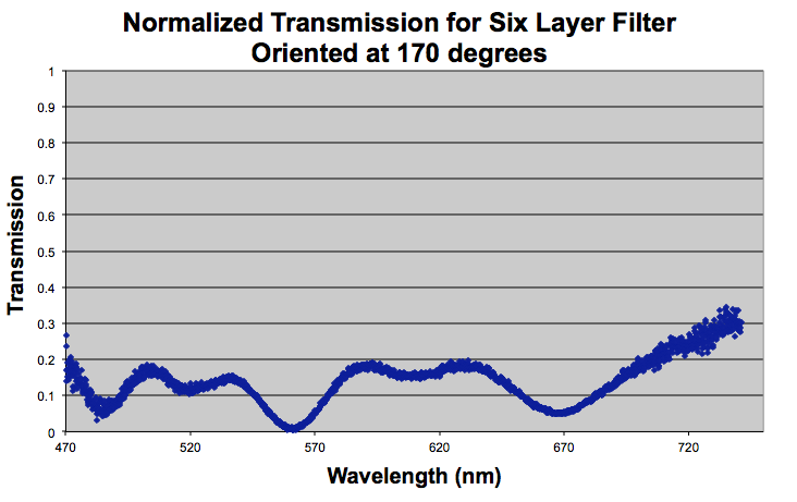
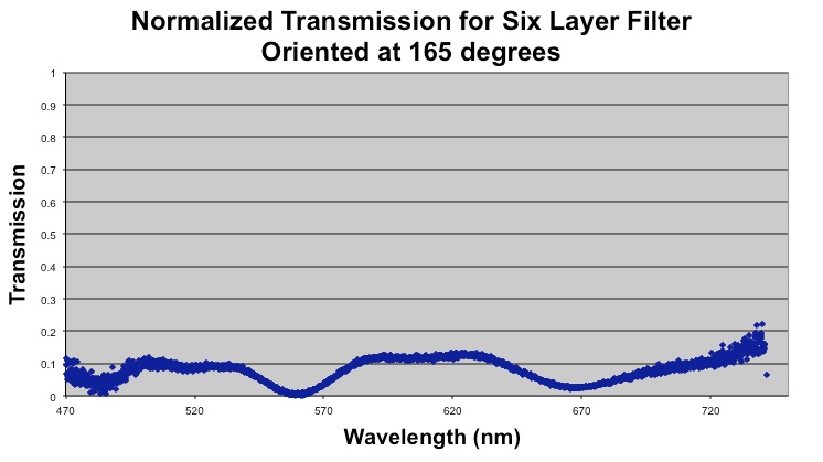
In the graph, the dips between the original wavelengths for QWPs are the original maxima of the six layer sample. Here, they dip and don't match up vertically with the QWPs. Since the filters I'm using (strips of cellophane tape) aren't exactly perfectly homogenous, the theoretical theta value didn't work perfectly to create a QWP. It did get me significantly closers, since I don't see huge oscillations anymore, but I still need to increase the retardance. For the rest of the day, I played around with the rotation angle, and found that 165 degrees produces a retarder extremely close to that of a QWP! Since I knew I had to increase the retardance to get the flat curve, I moved rotated the filter closer towards its fast axis. The final normalized data is shown below:
August 4, 2014
It's our last full week of research! I cannot believe how quickly this summer has flown by! It feels like just last week were learning about the pig toy and burning paper with lenses outside.
I started this morning off at the whiteboard explaining to the rest of the lab Malus' Law and showing them the Jones calculus derivation. Melia also talked to us about posters. They should be done by this Friday, so towards the middle of this week I'll start gathering all the graphs I've made and the data I've taken over the course of the past month and half.
After, I went straight to my computer to figure out how to make the quarter-wave plate (QWP) from the pieces of tape. Using mathematica, I was able to write a series of Jones matrices to solve for the angle theta that I should be able to rotate the pieces of tape relative to each other to align the slow and fast axes of the retarders to create a QWP. I found that the angle should be either 170 or -170 degrees. I'm really excited to see if this actually works, especially since I haven't been able to find any literature online or in published journals about making a QWP from a half-wave plate (HWP), particularly those made from pieces of cellophane tape.
I spent the rest of my day reading more on QWPs, since I want to be sure to know what to look for when I actually create the filter and writing all my exciting progress in my research journal.
August 1, 2014
I can't believe it's August already! My project is winding down, as I finished normalizing the waves for 2, 4, 6, 8, and 10 layers of tape today. Since I've characterized the retardance of the tape (half-wave plate), I'm now going to work with Mathematica to see how I can arrange the pieces of tape to form a quarter-wave plate and other types of retarders. Hopefully I can create circularly and elliptically polarized light with the tape next week. After some playing around with the tape some more, I spent the rest of the morning learning Mathematica. Knowing how to operate on this program will be crucial to my creating the theoretical model for the tuneable filter I hope to create, since I'll be calculating a number of Jones matrices at a time.
July 31, 2014
Today was a writing day. I did a lot of writing in my research journal, online, and for my abstract. I even started brainstorming ideas for the title of my project. I was also able to normalize the waves for four layers of tape and observed that the waves were a lot more rounded, probably because the light goes through less rotations as it goes through the filter, and there were less maxima/ minima.
July 30, 2014
Today was an extremely eventful day. Because the LTC students were going to be presenting at the pizza lunch, we didn't have a morning meeting; instead, we worked on our PowerPoint presentations. The presentations were intended to be a quick update on our progress thus far with our projects and overall research experience here.
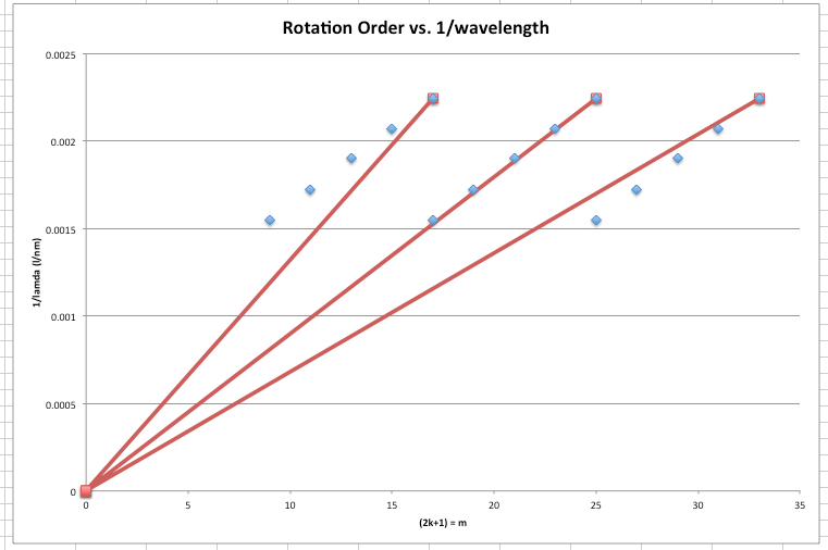
Before the presentations, I worked on the k-plot Dr. Noé had suggested I try to graph. Even though I was able to determine that the tape is a half wave plate, due to the clear extinctions of light at the minima (where the intensity equals zero), it wasn't apparent what order, or what odd multiple of pi, the ten layers of tape actually were. Using the retardance equation (below), we were able to figure out that the odd multiple of pi, m=(2k+1), was 17, making the ten layers of tape the eighth order of rotation.
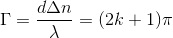
Mathematically, when m is zero, 1⁄lamda is zero, so graphically the line of the k-plot on a graph of m vs. 1⁄lamda should pass through the origin. Only the points of the proper order of rotation passed through the origin, as shown in the graph below.
After presentations, I wanted to work on normalizing ten layers of tape between two crossed polarizers. Since retardance is dependent on wavelength and the way in which the light was being polarized differed with two crossed polarizers, the wavelengths at which the films would be half plates would also shift. After collecting data on the intensity of light transmitted through the filters, I followed the same procedure to normalize the waves as I had with the parallel polarizers. After several attempts to normalize the waves and countless re-checkings of my data, I still seemed to get curves that resembled Lorentzian curves, rather that the sinusoidal curves I had expected and gotten with the parallel polarizers. After a lot of thought and discussion with Dr. Noé, Marty, and Melia, I realized that my incident light had been recorded improperly. The incident light when graphed had oscillations, something that should not have occurred. I re-recorded data for the incident light and then applied that to the data for both the parallel and crossed polarizers. At the end of the day, my final normalized graphs looked like this:
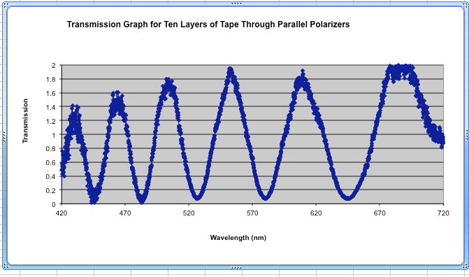
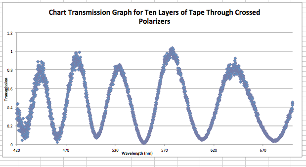
As shown, the graphs are complete opposites of each other. Where there are peaks for the parallel polarized, there are minima for the crossed polarizers and vice versa.
July 29, 2014
At the whiteboard meeting this morning, it was Andrea's turn to teach a lesson. She demonstrated the connection between pressure and sound, a phenomenon she will be working very closely with for the rest of her project. Overall, I think it's been really cool to have a student teach a lesson each day because we really get to know what others are working on and learn so much in the process. Looking back, I don't think I realized how much I could learn in one summer. I'm definitely getting a bit nostalgic since the summer is coming to an end, but working at the LTC has truly been an amazing experience.
The rest of the day was spent trying to normalize the waves for ten layers of tape in between two parallel polarizers. Since the oscillations in the graphs for ten layers of tape were a lot greater, due to the increased number of rotations, I decided to start with it for the process. I figured since I would have to do some math to normalize the waves, it would be best to use an excel sheet to graph and chart my data. On the ThorLabs analyzer program, I figured out that I could export the graphs as a series of coordinates in a text file that could easily be copied into excel. By the end of the day, I was finally able to generate a normalized graph of ten layers of tape in between two parallel polarizers (below) by dividing the output by the incident light. At first I was considering the incident light to be the light going through just one polarizer, but I realized that due to absorption, it would be more acurate to consider the incident light as the light transmitted through two parallel polarizers. It was diffcult to determine a formula to normalize the vectors because a paper I had read earlier used a completely different, more vague method.
We also sat down with Dr. Noé in the conference room to discuss the basic structure of abstracts. Since we will have to submit them soon, Dr. Noé wanted to make sure we understood the basic format of an abstract as well as what we needed to include in it. We brainstormed keywords to have in our abstracts for each of our projects and also came up with possible titles for our posters and papers.
July 28, 2014
Today Jonathan started off the morning by giving us a quick introduction on the Fourier transform and its applications in optics. When Dr. Noé arrived, I sat down with him and Melia to discuss in more depth the direction of my project. Like every research project, mine has been constantly developing and shifting in methods. We decided the first step in my project, now that I have been exploring the general ideas of polarization and retardance for a few days now, would be to determine the specific retardance of the filters I am using. In order to do that I would have to determine the transmission of the light by figuring out how to normalize the waves being read from the spectrometer. After, Dr. Noé suggested the idea of "tuneable retardance." He asked if it would be possible to create a quarter wave plate or different types of retarders by rotating the filters relative to each other. I really liked the idea, and I think that will be the final direction for my project. Ultimately, I hope to create a tuneable birefringent filter that produces different types of polarized light.
For the rest of the day, I played around with the idea of normalizing the waves and different layers of tape. When I recorded the intensity vs wavelength for 4, 6, 8, and 10 layers of tape between two parallel polarizers, I got beautiful oscillation patterns that display the extinction and transmission behaviors of the tape. I now have to figure out how I will normalize the waves to determine the retardance of the wave plates.
July 25, 2014
Today I spent the day at Brookhaven National Laboratory exploring and listening to lectures from various reseachers at the facilities with the rest of the Simons fellows. It was super fun!
July 24, 2014
This morning Alex helped us finish the derivation of the equation for the intensity of the diffraction pattern at a certain point P in the double slit experiment. I then spent the rest of my day applying Jones calculus to the Law of Malus and creating a project plan for the next couple weeks.
Malus' Law basically states that when completely polarized light is incident on an analyzer, the intensity of the light transmitted by the analyzer is directly proprtional to the square of the cosine of the angle between the transmission axes of the analyzer and the polarizer. Since the majority of my project deals with the polarization of light, the Law of Malus is extremely crucial to understand as a foundation for my learning. Before setting off to derive this mathematically through Jones calculus, I wanted to see this law in action, so I set off to do some experimenting.
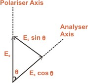
Basic diagram displaying components used to derive Malus' Law.
In order to derive this Law experimentally, I fixed a linear polarizer to the light of an overhead projector and rotated another linear polarizer at increments of 15 degrees from 0 to 90 degrees, measuring the intensity of transmitted light at each angle. The data I collected is shown below.
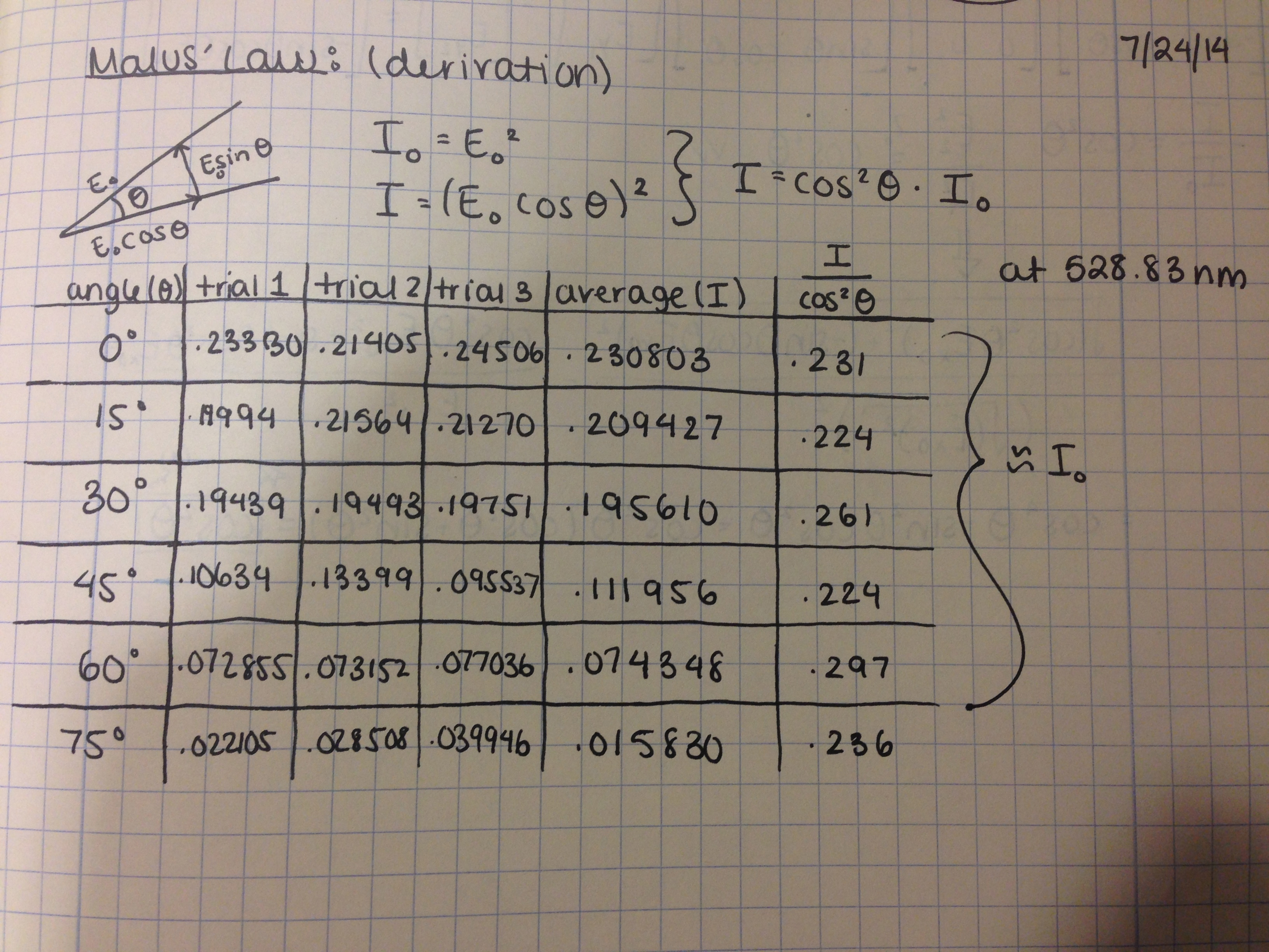
Since according to Malus' Law, the intensity divided by the cosine squared of the angle between the transmission axes is equal to the intial intensity, we should have gotten values closed to about 0.23. Looking at the data, that's about what I got for all the ratios calculated. Of course, not all measurements were extremely precise, but this was a good introduction into the experimental world of polarization.
After the experiment, I was able to derive Malus' Law using Jones calculus by setting up a series of matrices representing the experimental set up. Hopefully I can present what I was able to figure out on my own to the rest of the lab at a morning whiteboard meeting.
Today I also got the chance to sit down with Melia to come up with a potential project plan for the rest of the summer. Basically, using my knowledge of Jones calculus, I now want to build a basic mathematical model of the birefringent filter to predict the type of light that will be transmitted. From there, I want to build the filter and collect data. Upon analyzing my data, I'll be able to tweak the math model I came up with initially and then apply the pressure component to the theoretical model (for a tuneable filter). Then I can build the tuneable filter and compare my real data to the predicted results.
July 23, 2014
Today was a learning day. I started off the morning today at the whiteboard giving the rest of the lab an introduction to Jones calculus. I explained the basic Jones vector (below) and went through the derivation of the matrix for circularly polarized light.
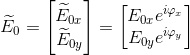
Jones vector used in many different calculations for polarized light, where phi represents the phase of the x and y components.
After deriving the matrix for circularly polarized light, the last step was to normalize it to a generalized form. When I first read through the textbook with the explanation of circularly polarized light, I didn't realize I had skipped over an important step in fully understanding the concept of normalization. In order to normalize a vector, the sum of the squares of the absolute values of the x and y components must equal 1. If they don't, we can divide the sum of the squares of these components by their reciprocal to get the normalized matrix. The general form of circularly polarized light in Jones calculus looks like this:

In order to normalize, we take the sum of the squares of the absolute values of the x and y components:

If I continued the derivation with my understanding of the bars as absolute value signs, I would have gotten zero. In reality, what we're really looking at are magnitudes. Where the absolute value of i2 is -1, the magnitude of i on the polar coordinate system is 1, making |i|2 equivalent to 12, or 1. Using this approach, I got the normalized vector for circularly polarized light to be:

After our meeting, I decided to focus more on the math part of my project and do some problems with Jones calculus. Below is a basic example of a problem I did in which I had to normalize and characterize a vector:

Normalized, the vector is multiplied by the reciprocal of the x and y components' magnitudes sqaured to produce linearly polarized light at -45 degrees.
Other questions I did included finding the angle between two polarized planes given E1 and E2.
After doing some math, I played around more with the spectrometer. The clear cellophane tape Dr. Noé had originally bought for me didn't seem to work so well in terms of displaying colors through linear polarizers. When rotating the analyzer, the tape only seemed to show black and white, possibly because it is so birefringent, the oscillations of intensity vs wavelength occur too quickly for the changes in color to be visible. I then played around with the different types of tape we had laying around in the LTC, and I stumbled upon packaging tape. The changes in color were extremely beautiful and visible enough to see with the naked eye. For the rest of the day, I played around with different layers of tape, observing the changes in color and intensity with the spectrometer.
July 22, 2014
This morning Libby showed us a derivation of the equation for the dark fringes in the single slit experiment (diagram below). Using the equations for the electric field generated and the intensity function, we were able to come to a pretty clean equation.
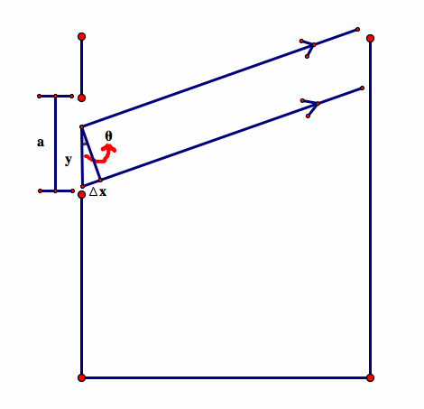
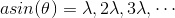
Final single slit equation for dark fringes.
After our meeting, I started playing around with the spectrometer. Using different colors of LED lights, fluorescent bulbs, and a HeNe laser, I was able to measure the intensities of different wavelengths present in all the types of light. Through this, I was able to gain a better sense of the analyzer software, figure out how to specifically measure the peaks of waves, and understand how to analyze the graphs produced. Images of the graphs for the lights I tests are linked on my spectrometer page.
July 21, 2014
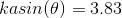
The spectrometer from ThorLabs arrived today! Before that, in the morning, though, we finally were able to derive the "1.22" from Rayleigh's criterion (with help from Melia, of course...). The radius of the first bright spot ends at the first dark ring. At the first dark ring, the intensity of light is zero, so using the Airy equation for intensity, where k is the wave number, a is the radius of the circular aperature, and J1 is the first order Bessel function:
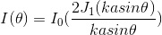
we have to find a value of the first order Bessel function equal to zero. Looking at the graph of the function, we see that the first zero is equal to 3.83. So plugging in, we have:
Substituting the wavenumber for its extended value, we can solve to get the constant 1.22.
After our morning meeting, I read more about Jones calculus. I'm thinking about doing a morning lesson some time this week on Jones matrices.
After some reading, I began building my optical setup for the birefringent filter. Right now, I'm trying to build a simple setup without the pressure component to get some base readings. I started putting together the polarizers and playing around with the spectrometer. Unfortunately, the analyzer software only works on PCs, so I can't use my own computer. For now, while I get used to using the spectrometer and the software, I'll be using the PC in the lab away from my work setup.
July 18, 2014
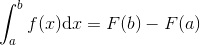
Today was a writing day. I did a lot of catching up in my research journal and spent time editing and adding pictures to my online journal and index. This morning at the whiteboard we learned about definite and indefinite integrals. An indefinite integral is essentially the anti-derivative of any function, which we are able to find by doing the inverse of the exponent short-hand rule. We also covered a definite integral, which has an upper and a lower bound. The mathematical definition is written out below, where F denotes the anti-derivative of a function at a particular point:
In the afternoon, Dr. Noé showed us a proof for double-slip diffraction on the white board. I also made organized the list of things I had to do over the weekend including finishing the chapter in "Introduction to Optics" on Jones calculus, reading more about birefringence and polarization, and understanding how to use the spectrometer.
July 17, 2014
Diffraction pattern of circular aperature when a screen is placed relatively close to the aperature.
Today was quite an eventful day! We started the morning at the whiteboard as usual, except instead of Melia teaching us a lesson, each of us were asked to go over or review a concept. Each of us took a piece of scrap paper and wrote down about 8-10 things we knew about optics or had learned the past couple weeks (I went a bit overboard and wrote 14...whoops!), and then passed the sheet to the person to the right of us. Our neighbor then circled the concepts they wanted to go over or didn't know and wrote those on the board. Each person then had to teach the rest of us the concepts or equations that were circled on his or her sheet. I really liked this activity because the majority of the concepts circled were those that related to each person's specific interests and research. I talked about birefringence and polarized light, while Libby taught us about integrating spheres and oximetry. Andrea showed us how an acousto-optic modulator works, and Jonathan explained the lens aberrations he has been looking into. We were also able to review concepts we had learned earlier this summer but had just forgotten or never fully understood. Alex reexplained Euler's formula (below) and why certain lenses cause paper to burn (explained in previous journal entry from June 30, 2014).

Note: In the LTC the zero in Euler's formula is actually a smiley face :)
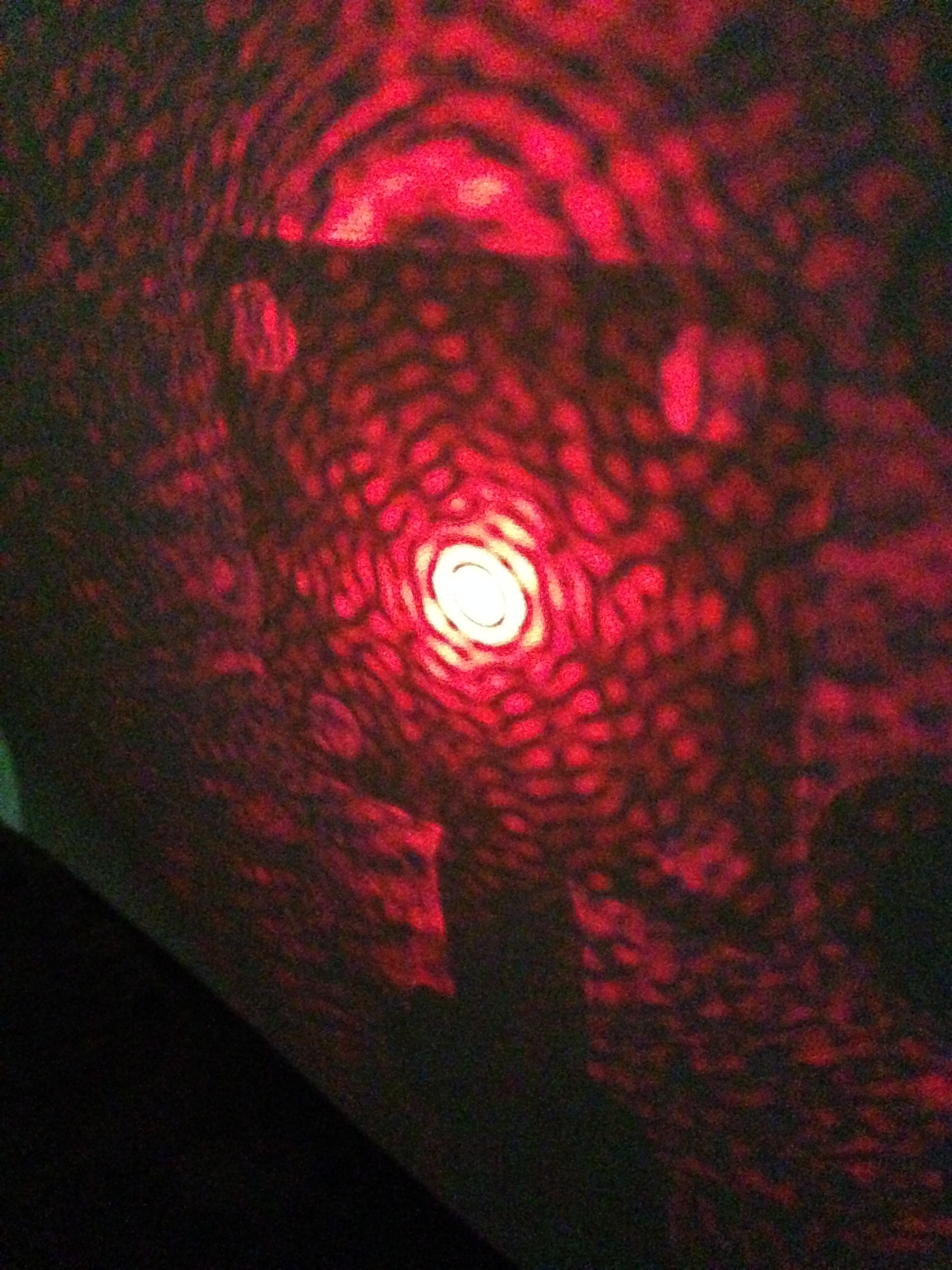
After our whiteboard meeting, we went to the back of the lab to mess around with some diffraction patterns. A lot of this was our just getting used to how certain equipment, like the lasers, works and building setups. When we couldn't at first get the laser to go exactly through the circular aperature, Dr. Noé exclaimed, "Welcome to research!" In a lot of our experiments, we will encounter diffuculties with equipment and trouble with setting up machinery, and this mini-project was a firsthand example of such. For the rest of the afternoon, we played with circular, triangular, and square aperatures to observe their diffraction patterns (images below). Using Rayleigh's criterion for a circular aperature, we were able to make measurements to determine the wavelength of the red laser. Knowing its wavelength was 632 nm, we came pretty close to that using a 200 micron circular aperature, with our final result as 615 nm. When we conducted the experiment again with a circular aperature of 500 micron diameter, our margin of error was significantly larger. We aren't exactly sure why we were so off with our measurements, but I have a feeling it has to do with our measurement of the radius of the bright spot. Because it was a lot bigger, we got a little lazy with measurement and ending up rounding off or estimating most measurements.


From right to left, we can see the diffraction pattern for a square aperature, a circular aperature, and a triangular aperature. With each aperature, we can observe a certain symmetry. With the square we see diffraction gratings on each side of the square with a four-fold symmetry, with the circle we see rings with a circular type of symmetry, and with the triangle we see six sets of gratings with a three-fold symmetry.
After lunch, we heard about the terrile Malaysian Airlines plane crash in Ukraine. Dr. Noé was reading an article on NBC News about the incident and pointed out something fishy to us. Andrey Tarasenk, a miner who saw the explosion who was about ten miles away from the plane about six miles high, claimed to have seen a white trail go up from the ground and then heard an explosion two seconds later. We all know that the speed of sound is significantly slower than the speed of light, so how could someone almost 12 miles away from the plane itself have heard the explosion a mere two seconds after it occurred? Well, he couldn't have.
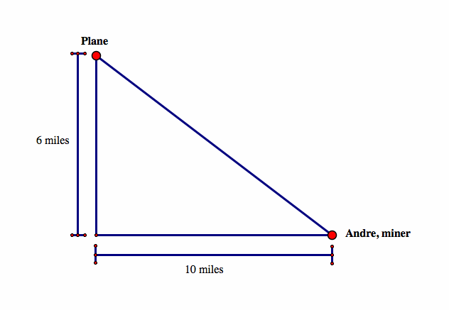
The speed of light is about 3x10⁸ m/s, while the speed of sound is about 340 m/s. This means that for someone twelve miles away from something, it would have taken him about 56 seconds to hear the explosion, not 2!
Another question Dr. Noé posed was how long it would take the plane to fall to the ground and compare that to what the miner reported. Neglecting air resistance, it would take the plane about 44 seconds to fall to the ground. The miner reported he saw smoke rising from the ground 10 seconds after he saw the plane explode, another fishy mismatch in details.
I spent the last hour of lab looking at Jones calculus. I asked Dr. Noé if I could take "Introduction to Optics" home, which has a great explanation of Jones matrices, and he said I could as long as I promised to write a solid entry in my research journal. I guess I have a long weekend full of Jones calculus ahead of me!
July 16, 2014
Today we presented our project proposals in front of Dr. Noé, Melia, Marty, and the rest of the lab. My full presentation is detailed on my project proposal page. We essentially discussed the direction of my project as I laid out the specifics of the physical and mathematical concepts I would cover and need to learn, along with the equipment required to undergo the project. With Marty, Melia, and Dr. Noé, we decided that to continue on the path of FBGs with an acousto-ultrasonic fiber optic sensor would be impractical because of time and resource constraints. Unfortunately, here at the LTC, we don't have access to ultraviolet light or tuneable lasers, something I would necessarily need to create the pressure sensor. Instead, with guidance from the three of them, I've decided to create a tuneable interference birefringent filter with polymer films that is sensitive to pressure. This project will cover a wide range of topics including polarized light and its interactions with birefringence to Jones calculus. I'm really excited to conduct research in this field because my project will allow me to go in a number of directions. In the past, physicists have been able to create birefringent filters using polymer films, although most have used more expensive, rare materials such as quartz, but, to my knowledge, no one has tested the effects of pressure on birefringence. If I were able to create a tuneable filter that were sensitive to pressure, I would basically be creating my own FBG using polarized light and polymer films. From there, I would be able to explore a variety of other phenomenons, including those of mirrorless lasers, the use of electro-optic materials to create birefringent filters, and applications to displays and color filtering.
Right now, I need to spend a bit more time reading up on polarized light, birefringence, and the effects of stress on birefringent materials. My research from UC Santa Barbara last summer, where I conducted a study on the behavior of non-Newtonian fluids under stress, will come in handy, although I won't be using any of my specific data for this project. I will also spend this weekend trying to understand Jones calculus and getting used to Mathematica so I can understand the math behind the physical phenomena, as well as try to form my own hypotheses before conducting any experiments. As of now, the only equipment I don't have access to in the LTC is a spectrometer that we will hopefully order tomorrow. I'm excited to start working on my project soon! I can't wait to see where my work takes me.
July 15, 2014
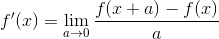
This morning at the whiteboard we learned about derivatives. Never having been exposed to calculus before, this was an extremely helpful lesson because derivatives show up in optics all the time. In addition to learning the basic and mathematical definition of them, we also did a derivation and then applied the equation (below) to several functions.
The rest of the day I spent reading about concepts related to my new project idea for birefringent filters. I'm currently reading a paper from the American Journal of Physics called "Interference birefringent filters fabricated with low cost commercial polymers" by Pablo Velasquez et al. to get a better idea of how to begin my optical setup.
July 14, 2014
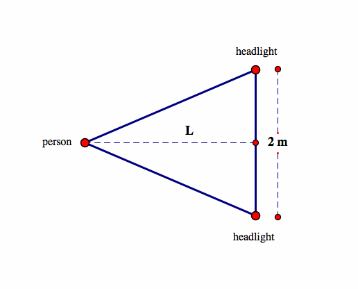
Today we began our day with a morning at the whiteboard. We solved another estimation problem that used key optical concepts such as diffraction and Rayleigh's criterion. Melia asked us how far we could be from a truck on a straight road to still be able to distinguish the two headlights.
First we established the two headlights and the person looking at the truck, whose eye serves at the diffraction apperature, as point sources with a diagram similar to this:
The basic problem arises from Rayleigh's criterion which explains that when two diffraction patterns are close enough to each other, we cannot resolve them.
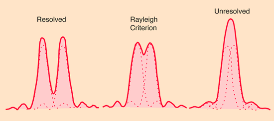
Since we are using a circular diffraction apperature, our eye, we use the equation
where D is the diameter of the apperature and lambda is the wavelength of the light we are seeing.
Estimating an average 500 nm for lambda and 5 mm for D, we use Rayleigh's criterion and the small angle approximation to find theta, which is about 1.22x10⁻⁴. Going back to the diagram above we can solve for L to get an approximation of around 6 km. This means that for a person with about perfect vision, he or she can be about 6 km away from a truck and still be able to distinguish its two headlights.
The rest of the day we hashed out some project plans and examined the practicality of each idea. When looking at my idea to build an acousto-ultrasonic fiber optic sensor, Dr. Noé pointed out the fact that obtaining the FBGs (which, to my surprise, aren't even manufactured in the United States), would take a long time to acquire and require a tuneable laser. I then looked into building my own and found out that I would need to obtain a license and an ultraviolet laser, neither of which I currently have access to in the LTC. I did speak to a representative from timbercom, a technology company based here in the United States, and he advised me to look into Bandpass filters. At the same time, Dr. Noé found a paper on birefringent filters, which related directly to my original interest in polymers and polarized light. Using pieces of scotch tape, the authors were able to create a bandpass filter. I was hoping to take this a few steps further in applying pressure to the stack of polymer films in order to tune the bandpass, somewhat mimicking the behavior of an FBG. By doing this project, not only will I be able to learn more about Jones matrices, polarized light, and birefringent filters, but I will also be able to adapt previously performed work in a manner related to my interests.
July 11, 2014
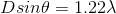
We started this morning with another simple problem on the white board: what is the average velocity of the earth travelling around the sun? Using Kepler's 2nd law, we established that a line segment joining the Earth and the Sun sweeps out equal areas during equal intervals of time (depticted below):
Even though the Earth's orbit is in the shape of an ellipse, since the velocity varies at different points on the path and we are trying to determine the average velocity, we can assume a circular path with a radius of the Earth's average distance from the sun. Using basic algebra, we were able to determine that Earth's average velocity is about 30,000 m/s.
After our whiteboard session, there was an AMO presentation in the conference room by a representative from the SAES Getters Group. A getter is a surface that traps molecules rather than releasing them at certain temperatures, essentially serving as a molecule pump. The representative gave a clear presentation on the various pumps his company was selling and the advantages that came with them.
July 10, 2014
We started today with an estimation problem. Looking at a photograph, we were asked to determine the focal length of the camera that took the photo, without actually seeing the camera. Enrico Fermi, a famous physicist, is known for having solved many of these types of problems quickly and accurately over the course of his life. Some famous problems include how many piano-tuners are there in the city of Chicago or how many molecules per second we breath in of Fermi's last breath.
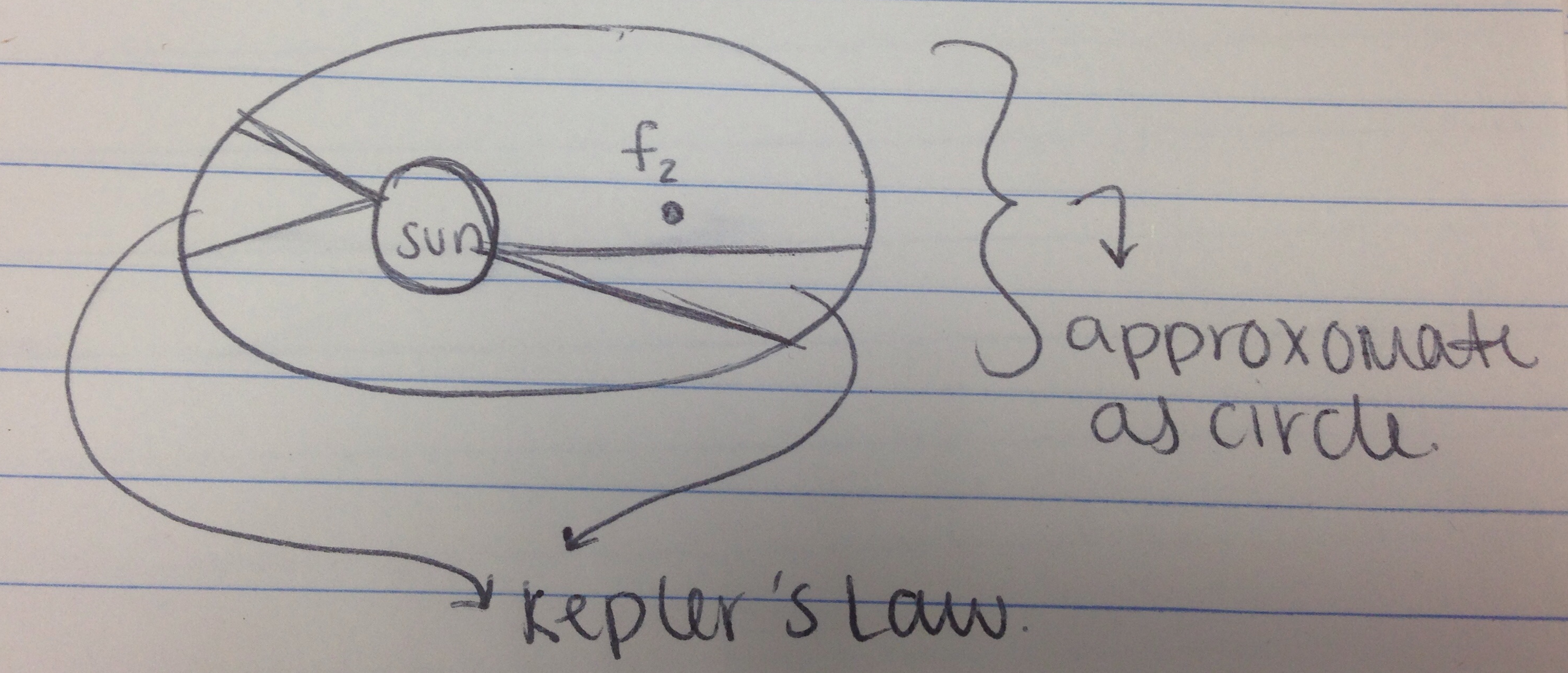
We started the problem by drawing a diagram of what the camera forming the image looked like.

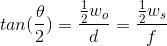
We decided to solve the problem by looking at the widest object the camera could capture in its frame of view. We established that it was the court and bleachers. Its width is labeled wo. The wide angle that the light comes in with for that object is the same angle that the light defracts to form the image in the sensor, essentially forming similar triangles. Since we are looking at the widest object the camera can capture in a shot, the width of the sensor is equal to the width of this object in the image, labeled ws. Since the image is formed in the sensor, where all the light meets to form the image, the distance of the lens to the sensor is the focal length. We also noted that the axis of symmetry bisects the angle theta present in both triangles.
Using basic trigonometry, we were able to establish that:
From there we were able to establish a simple ratio with values we could assess.

In order to determine the dimensions of the court and the bleachers, we were forced to estimate. None of us knew at the top of our heads the dimensions of the average tennis court, nor were the dimensions given to us previously. In the bleachers though, there were seats that could fit the average person. We estimated the average width of a person and then counted (about) the number of seats per bleacher. From there we were able to get wo and d, the distance from the lens to the object (which we assumed to be from the corner of the court to the midpoint of a diagonal). We then had to estimate the size of the sensor, which we took to be about 2 centimeters. In the end, we got a focal length of 10 mm, which is actually the exact focal length of the camera that took the image.
I spent the majority of my day reading about the Fourier transform and its applications. I met with Marty about my idea for the acousto-ultrasonic fiber optic sensor, and we discussed how I could potentially use the Fourier transform in the analysis stage. During our meeting, Marty, Dr. Noé, and I read over Betz' paper (cited in an earlier journal entry on July 3, 2014) on his use of acousto-ultrasonic waves for fiber optic sensing. The first step in building my sensor for non-invasive medical techniques is acquiring the FBGs. Using an FBG that is able to reflect visible light and a tuneable laser, I will hopefully be able to build a sensor that can detect pressure changes in the human spine. An issue I may encounter in the detection process stems from the fact that pressure changes in the human body remain static post-drip. Since the pressure will not be constantly fluctuating in the human spine, and I am trying to measure the change in pressure and not just a given quantity of pressure, I will have to figure out how to use sound waves to detect the a change in pressure.
July 9, 2014
The presentation/ discussion with Professor Metcalf went very well today! Although I definitely could have pitched in a bit more, I enjoyed being able to talk about laser cooling, a process that interests me very much. Before the meeting, Dr. Noé and Melia had each of us go over a few concepts to brush.
Since we went over resonance and the Q factor last night before leaving the lab, we went straight into discussing simple harmonic motion (SHM). The basic equation for the force makes use of "k," which, in the case of a mass attached to a spring, is the spring constant.
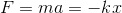
Taking the second derivative of the equation for force we get:
Because the displacement graph of the motion represents a sine wave with a variable angular frequency, we can combine that equation (sin(wt)) with the one above to get omega, the angular frequency, as:

We also talked about the Lorentz curve (pictured below compared to a Gaussian curve):
The equation for the curve is written out in an earlier journal entry (July 3, 2014).
We also mentioned the Doppler equation which can be written as:

The Doppler shift is particularly important in discussing laser cooling, as physicists have to account for this shift in frequency when trying to match the frequencies of laser beams with those of the atoms.
During my discussion with Professor Metcalf, we went over the basics of temperature and kinetic energy before diving into the more complicated processes of laser cooling and Bose-Einstein condensates. I was finally able to answer the question about when a baseball is thrown, given that we know that kinetic energy and temperature are directly proportional, why it doesn't get hotter. In a baseball where all the atoms are travelling in the same direction and at the same speed, the velocity of the atoms are the same relative to each other. Because of this, while the kinetic energy of the entire system has increased, the kinetic energy of the atoms relative to each other hasn't, so the temperature does not increase (since we know that kinetic energy is temperature multiplied by half of Boltzmann's constant). We also discussed the differences between quantum mechanics and classical physics, and when we would use one over the other. Generally when we are looking at single particles, or things that can't be broken down any further (like electrons), we use quantum mechincs. For composite particles, we use classical physics.
After, we had the pizza lunch. One student working in Dr. Allen's lab talked about his work on analyzing the work of Professor Koch of Stony Brook on a two-dimensional minicrystal structure of seven steel balls. He examined the trajectories of the balls based on the normal modes of the system. Taylor Esformes, a graduate student at Stony Brook, talked to us about hyperspectral imaging and its various practical applications. Then Marty talked to us about his efforts to try and achieve clearer imaging for BECs by using a diffuser and scattering the light of the laser beams.
July 8, 2014
Last night after lab hours I spent more time thinking about acousto-ultrasonic fiber optic sensors and their practical applications for a potential project. After talking to my mom, a physician, I discovered that many medical tests use invasive techniques. For example, when one develops a brain infection, there is a fluid build-up in the cavity that drips down to the spine. In order to determine whether or not the patient actually has an infection, physicians insert a needle into the spine, and the pressure with which the fluid comes out serves as an indicator. Not only is this an invasive method, but also is a crude measurement of pressure. Using acousto-ultrasonic fiber optic sensors could be a non-invastive solution to this issue. Since sound waves are essentially pressure waves, we could potentially build an acousto-ultrasonic fiber optic sensor using my knowledge of various optic sensors to non-invasively detect pressure.
After our morning meeting where Melia told us to start thinking about topics for mini lessons we would be doing throughout the rest of the summer, I decided to look into polarized light as a possible lesson topic. Although for my project I hope to do something in acousto optics or laser cooling, I am still interested in polarized light and its overlap with polymers, so I may decide to teach a lesson on something I find interesting in this field.
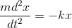
Light can be represented as a transverse electromagnetic wave with fluctuating electric and magnetic fields. Light is seen as having three axes, the x typically representing the velocity of the wave or the direction of its propagation, the y representing the electric field, and z the magnetic field.
The picture on the right displays the electric field vector as the wave propagates through space.
Linearly polarized light contains waves that only fluctuate in a specific plane. It is a special case of circularly polarized light, when the two waves propagting in the XY- and YZ- planes are in phase.
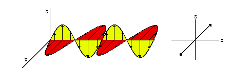
If the two waves are 90 degrees out of phase, the resulting wave is circularly polarized, which essentially means that the resultant electric field vector rotates around the origin as the wave propgates.
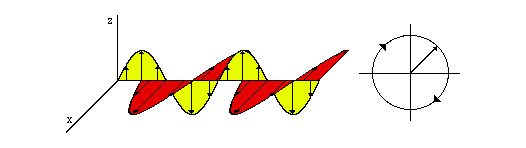
The most general case of polarized light is when the phase difference is at an arbitrary angle, so not 90 or 180 degrees. This is called eliptical polarization because the electric field vector traces out an ellipse, as compared to a line or a circle.
Today I also read Jenny M. Smith's paper on her "Polarized Light Examination of Oriented Polymer Films." Her paper basically described one of the overlaps between polymers and polarized light, something I had come into the LTC very interested in. She began her paper by descrbing the process of orienting films, which ultimately gives polymers a greater toughness and tensile strength, altering their optical properties. The process itself is essentially a series of controlled heating and coolings and drawing and stretchings of the polymer chains, bringing them out of their amorphous state.
There are three refractive indices (RIs) in these crystalline films:
1. nmd: RI in the machine
direction (along the length)
2. ncd: RI in the cross
direction
3. nfm: RI normal to the
plane
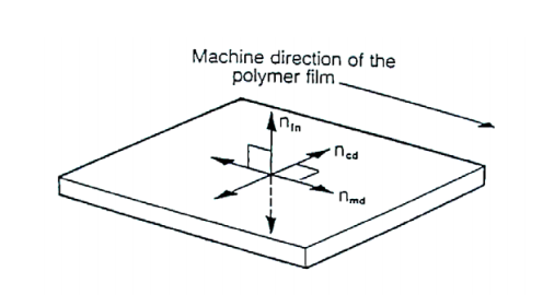
Because of the three orthogonal RIs, the polymer is able to behave like a biaxial crystal.
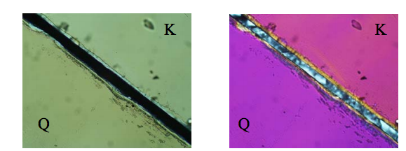
Viewing polymers under polarized light (plane/crossed), we are able to better understand the optical properties of the films. For example, if the sample is completely dark under the crossed polars, the polymer is isotropic and non-crystalline. If patterns are visible, the film is anistropic and crystalline.
Retardation, essentially the color of polymers under cross polars, is a funciton of the birefrigence and thickness of the polymer itself. The images below display these differences.
Sources used:
"Polarized Light Microscope Examinations of Oriented Polymer Films" by Jenny M Smith et al (paper)
I also met with Professor Metcalf to discuss laser cooling. Tomorrow Dr. Noé was hoping Professor Metcalf and I could lead a discussion on the process and give a little background to the issue. Professor Metcalf gave me the first three articles ever published on laser cooling from the Scientific American, which includes one he wrote himself. I'll be reading those tonight for our discussion tomorrow.
July 7, 2014
This morning we went straight to the white board to do a derivation of the golden ratio. If we took a standard segment and split it into two parts, calling the longer segment a and the shorter segment b, the golden ratio would exist if the following equation held true:
In order to derive the actual value of the golden ratio (which we already know to be the irrational number phi=1.618...), we solved for a.
Solving for the ratio we get:
We can ignore the negative value from the equation because we are looking at measurements (only positive values).
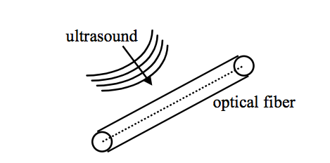
I started work right after by reading a paper by Pavel Fornitchov et al on "Fiber Optic Ultrasound Sensors for Smart Structures Applications." The paper introduced the benefits of fiber optics sensors as compared to piezoelectric transducers and established that optics sensors can take higher temperature measurements and are smaller in size and lighter in weight, compatible with composite materials, and immune to EMI. For their project, the physicists at Northwestern University used ultrasonic energy to interrogate fiber structures for damage. The sensors were used to detect ultrasonic energy after it interrogated the full structure. This not only allows for a relatively sparse distribution of fiber sensors around the structure, but also provides greater sensitivity in detecting small flaws because the energy is dictated by wavelength, rather than the spacing of fiber sensors themselves.
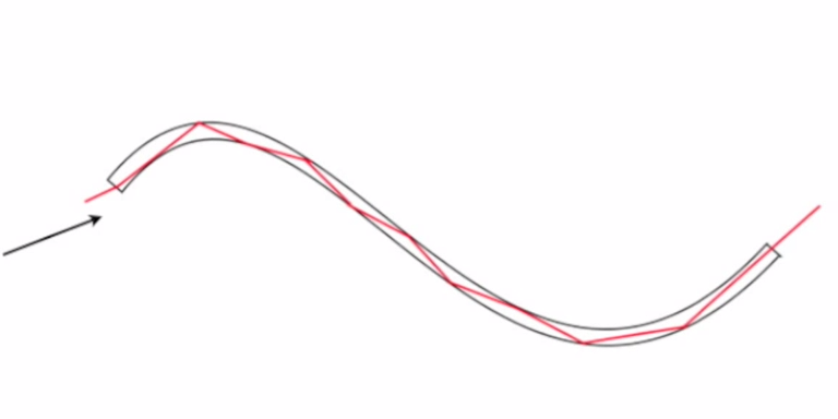
Below is a basic image of how ultrasound affects light propagating insides a fiber. Essentially, the ultrasounds causes a strain in the fiber, which affects the optical tranmission in the fiber in number of forms (i.e. dimensional changes, change in the refractive index of the fiber, etc.)
As described in Fornitchov's paper, in order to develop the sensor and complete their project, the physicists had to fabricate the fiber sensors and then build a sensor stabilization control system to help maximize and clarify the data they hoped to record. There were several sensors discussed including Fabry-Perot sensors, Sagnac ultrasound sensors, and FBGs. Sagnac sensors are noise insensitive and easier to fabricate than Fabry-Perot sensors, while FBGs are local sensors that are easy to make and easy to multiplex several of them in one fiber segment, although there are several issues with frequency response.
Sensors rely of frequency response to collect data. In elastodynamic analysis, we can calculate strain in the fiber core with the impinging ultrasonic wave. Strain-optic relations, another way of characterizing sensors, calculates the induced phase shift in the fiber sensor also when the impinging ultrasonic wave creates strain. The phase-shift induced by ultrasound can be calculated by the following equation, where the numerator is the ultrasonic signal voltage, gamma is the fringe visibilit, and V0 is the quadrature offset voltage:
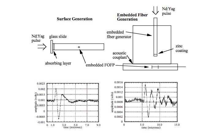
Acousto-ultrasonic fiber optic sensors have a variety of applications from detection of flaws, to acousto emission detection, to curing the monitoring of composites. For the future, Fornitchov et al recommend looking into fiberized laser-generation of ultrasound, which sounds very interesting (although I still have to look into it, as I don't know much about it at the moment). Below is a visualization of how fiberized ultrasound laser-generation might benefit us.
I also finished reading Daniel C Betz et al's paper on "Acousto-ultrasonic sensing using fiber Brigg gratings." Acousto-ultrasonics requires two probes to work efficiently: the first being an introduction of the ultrasonic stress waves into the structure and the second the pick up of these stress waves at another position. Betz and his associates wanted to create a sensor that would effectively detect damage on bigger machines, such as airplanes. The presence of damage is identified when the detected ultrasonic signal deviates from the reference signal of the undamaged structure.
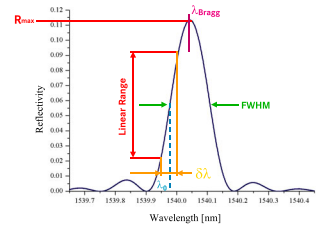
FBGs can be useful because they can detect both strain-based loads and acousto-ultrasonic damage. FBGs are essentially permanent, periodic perturbations of the refractive index which is laterally exposed in the core of an optical fiber. It is characterized by its period, amplitude, and length and acts as a filter for light traveling along the fiber, reflecting light in a predetermined range of wavelengths. The following is an equation for the Brigg wavelength, where neff is the mean effective refractive index in the grating region and gamma is the grating period:

External forces such as strain, pressure, and temperature lead to changes in the grating period and effective refractive index.
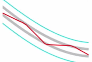
Generally speaking, ultrasonic acoustic detection has a higher frequency and smaller strain (usually at the micro-strain level) than other methods of detection. If the wavelength of the laser matches a certain part of the grating system, any shift of the spectrum will modulate the reflected optical power. The interrogation method used by Betz and associates concentrates on the part of the spectrum where the function is assumed to be linear. Below is an image of what this looks like.
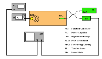
The set up used in this experiment (pictured below) allows for the monitoring of a large area of a structure with only one optical fiber and one ultrasonic transducer, making it different from sensors used before.
Sources used:
"Fiber Optic Ultrasound Sensors for Smart Structures Applications"
by Pavel
Fornitchov et al (paper)
"Acousto-ultrasonic
sensing using fiber Brigg gratings" by Daniel C Betz et al (paper)
July 3, 2014
Today we spent the morning continuing our research for project ideas. I finished the paper on laser cooling and am really fascinated by the idea of using light to cool atoms. I spent the rest of my morning until the RCR training reading up on other ideas listed on my ideas page, specifically laser cooling and acousto-ultrasonic fiber optic sensors.
The first of the two I spent my time on was laser cooling. Using Mark Kasevich and Steven Chu's paper on "Laser cooling below a photon recoil with three-level atoms" and a couple youtube videos (cited below), I was able to better understand the concept of such a phenomenon. Originally when I thought of lasers, I used to think of something that would produce heat using the light it emitted; in fact, using the same properties of a laser, physicists have found that we are actually able to cool atoms of particular elements down to a millionth of a degree Kelvin! Simply put, if a laser beam, adjusted for the Doppler effect, can match the frequency of a moving atom, then the atom will be able to absorb the photon. But there is a lot more to that.
Heat directly correlates to the kinetic energy of a group of atoms. Since
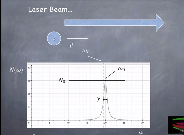
the ultimate goal in order to cool a group of atoms is to decrease the velocity of the given atoms as much as possible. When you place an atom in a strong laser field, it will produce a spontaneous photon, inducing a net momentum effect.
N, the number of spontaneous photons per second, is given as a function of omega (frequency):
Omega nought is the resonant frequency, while gamma represents the damping factor.
Since the laser frequency is doppler-shifted by about half of gamma, N has the largest slope at that point.
When a photon hits an ion, there is both a change in momentum in the direction of the laser beam and the spontaneous emissions (which is essentially random). The decrease in velocity can be more closely examined by the result of radiation pressure from the change in momentum caused by the laser beam, which produces an average force:
Since we have to use the Doppler-adjusted frequency:
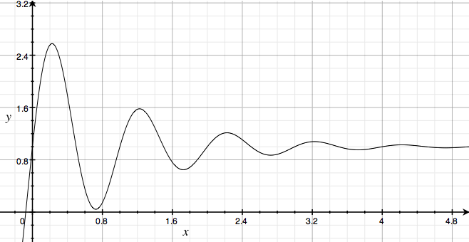
Applying the Taylor series, we get an equation for the average force which includes a damping effect directly related to the motion of the atom:
Because of the damper, we get this graph of the atoms motion or kinetic energy:
Sources used:
Laser Cooling - Sixty Seconds (video)
How Doppler Cooling Works (video)
Laser Cooling! - Steve Spicklemire (video)
"Laser Cooling Below a Photon Recoil with Three-Level Atoms"
by
Mark Kasevich and Steven Chu (paper)
The second topic I read up on was acousto-ultrasonic fiber optic sensors. Before understanding acousto-ultrasonic sensors, I first tried to fully understand fiber optics and how fiber Brigg gratings (FBGs) can be used as parts of optical sensors.
Using a very thin non-conducting glass or plastic fiber, a ray of light is shined through it such that there is repeated total internal reflection as the light travels the inside of the fiber. Because the angle of incidence equals the angle of reflection, the angle of incidence must be less than the critical angle for this phenomenon to occur. The fine fiber helps to ensure that this is so.
In many commercial fiber optic devices, the fiber is made of two materials with different refractive indexes in order to prevent scratching, or a leakage of light. The outer later of a lower refractive index protects the inner core and also allows for a gradual refraction rather than a sharp reflection.
For optical sensors, we often use FBGs. As white light travels down the fiber, it passes through an FBG, which is a series of optical filters that allows certain wavelengths of light to pass.
FBGs can be used to measure a range of factors including temperature and pressure. When there is a change in one of those factors, the FBGs compress or expand, allowing a different wavelength of light to pass. This allows physicists to maintain certain conditions in that particular environment.
I have started reading a paper by Daniel Betz on acousto-ultrasonic sensing, but I have yet to finish it. I also want to look into the idea of silicon photonics with fiber optic sensing.
Sources used:
Fibre optics (video)
Acousto-Optic Modulation for Sound Transmission (video)
FBG Optical Sensing Overview (video)
"Acousto-ultrasonic sensing using
fiber Bragg gratings" by Daniel C Betz et al (paper)
July 2, 2014
This morning we went straight into practicing presentations for the pizza lunch in the afternoon. Each of us practiced our full presentations in the conference room and Meilia gave us feedback on what to improve. All of us presented including Libby and Melia. After, we looked more into project ideas. I’m really fascinated by the idea of acousto optics, and I’ve been reading papers online including Graham Wild and Steven Hinckley’s paper on Acousto-Ultrasonic Optical Sensors. Dr. Noé had mentioned the idea of laser cooling on the first day as well, and I’m currently in the middle of reading a paper by Mark Kasevich and Steven Chu on “Laser Cooling below a Photon Recoil with Three-Level Atoms.” I am also considering a project on liquid crystal lasers and polarized light, inspired by an article I read in the Physics World magazine.
July 1, 2014
We spent this morning finishing up and editing presentations for the pizza lunch tomorrow. I’ll be doing a presentation on my work in the fluid mechanics lab at UCSB last summer. I went over my presentation with Melia and we made a few edits to my PowerPoint. I’m going to try and talk to Dr. Noé and Melia later today to discuss potential projects with acousto optics. I’ve been reading up on it, and I would really love to explore it even more. I also want to see what I can explore with polarized light and polymers. After editing my abstract for my presentation with Dr. Noé, I began looking at several project ideas in more depth. When reading about acousto optics, I read about how further research into the field could yield useful applications in nondestructive testing. I’d love to look further into that and explore the options of that as a project. Within acousto optics I could explore optical measurement of ultrasound to produce non-contact images, acousto optic modulators, or acousto optic deflectors and how they could potentially trap small molecules. Another project idea I was looking into is liquid crystal lasers and their relation to polarized light. I am also considering possibly studying diffractive waveplates or lasers that can overcome the Lorentz force.
June 30, 2014
Today was our first day in the LTC and a great introduction for the summer ahead. After the Simons reception where we met Dr. Noé and Melia, we headed straight to the LTC and instantly started playing with the pig toy. We established that because the image we saw at the top of the parabolic mirrors was a real image, if we shined a laser on it or looked at it through a magnifying glass, the effects would be the same as looking at a real, physical object. We also played with the idea of a sagitta and learned how it related to the radius of curvature and the focal point. After lunch at the Simons café, we went outside for a couple hands-on experiments. We used a polarizer to look at the effects of linearly polarized light on the sky, burned paper by focusing the light through magnifying glass to a small point, and examined the differences between various lenses and their f numbers and light gathering powers. We spent a lot of time at the white board after, discussing estimations, the small angle approximation, and the binomial approximation. Dr. Noé mentioned a possible project related to acousto optics and an acousto optic modulator, which really fascinated me. I’m definitely going to be looking more into that. We also looked at the effect of a polarizer with different polymer solutions, which was also really cool. We observed that the thickness and the physical orientation of the material itself affect how the light is polarized. We also looked at the interferometer in the LTC, which essentially splits up the light waves from a laser beam into two separate waves. Because there were two waves, we were able to observe and play around with the interference patterns, which were reflected on the wall adjacent to the apparatus. We used a rubber band to adjust the phase shift by one wavelength per second by slightly moving the mirrors, which appeared to change the frequency due to the Doppler effect.