Profiling a Gaussian Laser Beam
Ben Coe, Pradyoth Kukkapalli, and Annie Nam
Laser Teaching Center, Stony Brook University
August 2010
Introduction
Many people have the idea that laser beams are perfectly parallel "lines of
light." Initially, we also held this naive belief, but Dr. Noe challenged our
misunderstanding by demonstrating that the beam from a green laser pointer
clearly diverges. But how does the size of the laser beam relate to the
distance to the screen? We hypothesized that the beam width could not be
directly proportional to the distance because if that were true, extrapolating
back to a distance of zero from the laser would produce a beam size of zero,
which just didn’t make sense. We believed that the relationship would be
linear, but rather than being directly proportional the diameter and distance
would be related by an equation of the form ax + b, where a is the rate of
divergence and b is the initial diameter at zero distance.
This mini-project consisted of two parts. First, we looked at how the laser beam
from a green laser pointer diverges with increasing distance. This part of the
experiment was done in the long hallway outside the lab, where we could place the
laser as much as several hundred feet away from the screen. Later we measured the
intensity profile of a red HeNe laser by a much more precise method at distances
that were mostly less than one meter from the laser. Our results showed that the
profile is not linear as we originally expected, but rather is curved. The actual
hyperbolic shape is approximately constant near the laser and diverges in
proportion to distance in the far field, due to diffraction.
Green Laser in the Hallway
Our green laser was held on a small tripod stand that sat on the ground, and was
pointed at the wall at the end of the hallway. Each of us separately visually
estimated the diameter of the laser spot on the wall using a meter stick. We
repeated this procedure at several distances from the wall, from 35 meters (116
feet) up to about 141 meters (480 feet). We used a 25 foot tape measure to make
marks every 25 feet in the hallway to make measuring the distances more
convenient.
We plotted and analyzed our data in a spreadsheet program. We used the Least
Squares Method to determine the slope of the line of form ax + b that best matches
the data. This method works by squaring the difference between each corresponding
theoretical and experimental value. All of these terms are added together to
produce a measure of the total error. By minimizing the total error by changing
the parameters, we could find the curve that best represents the data points.
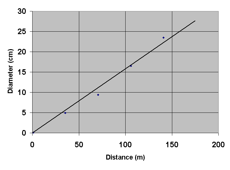
Figure 1. Estimated diameter of the green
laser
pointer beam as a function of distance.
The graph above shows our results. It is apparent from the graph that a line
passing through the origin (b=0) is sufficient to represent the data. We
realized from this initial experiment that we need to measure (profile)
the beam diameter much closer to the laser. The beam is very small there
so a more exact method is needed.
HeNe Laser Experiments
1. Razor blade method
We learned from different sources that the intensity distribution of many
laser beams is given by a Gaussian function -
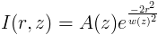
In this equation r is the distance from the center of the beam and A(z)
and w(z) describes the peak intensity and width of the beam, which both change
with distance z along the beam. I(r) can be measured directly by moving a
pinhole across the beam and recording how much light passes through it, as this past
LTC student did. Unfortunately one needs a very tiny pinhole or narrow
slit to get accurate results where the beam is very small. A better method is
to gradually cut off the beam by moving a razor blade into it, as shown in
this figure.
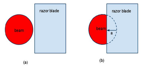
Figure 2. How a razor blade can "cut" a laser beam.
In this case the changing intensity of the part of the beam that's
not cut off is given by an integral like this, where x is the position of the
blade.
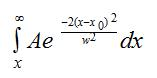
The theoretical curve given by this integral can be matched to the data points
by a least-squares method like we used before. The result is the width w of
the laser beam at some particular distance from the laser.
2. Setup and Procedure
Figure 3 shows our setup. We initially used the same green laser pointer as
before but unfortunately the characteristics of its beam suddenly changed when a
new battery was used, possibly due to damage to its crystal. Therefore we switched
to the very stable red HeNe laser shown. The photodetector was a Thorlabs DET110
whose current was read by a multimeter. We placed a converging lens ahead of the
detector to ensure that none of the beam missed the detector. As shown the
detector was intentionally placed away from the exact focus of the lens to avoid
possibly damaging the detector.

Figure 3a. A bird's eye view of the experimental setup
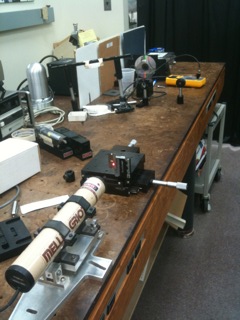
Figure 3b. A picture of the setup
The razor blade was taped to a right-angle bracket that was attached to a micrometer-driven translation
stage. We moved in steps of either 1 or 2 mils. (One mil equals 0.001 inch or 25.4 microns.) We made
these measurements at 31 different distances under 70 mm and also at 300 mm.
In all, we wrote down and entered over 1000 data points by hand.
In retrospect we took more data
than we needed. Fewer width measurements over more evenly spaced distances would have been sufficient.
3. Analysis and Results
Two types of analysis were done - (a) finding the beam width w(z)
at each of the 32 distances and (b) constructing the beam profile from these
results. Both used the least-squares method that was employed previously
with the green laser pointer data.
When finding the beam width by the least squares method one has the problem
that the theoretical function (integral of a Gaussian) can not be written
as a formula and thus cannot be directly compared to the data. The integral
in fact defines a special function called the "error function," or
erf(x). We dealt with this by numerically integrating the trial Gaussian
functions and comparing these numerical integral curves to the data. The
numerical integral is computed by simply summing all the Gaussian values
up to some particular point x. The result of one such least squares
analysis is shown in Figure 4.
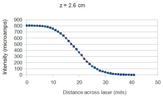
Figure 4. One of 32 sets of width data with its best-fit erf curve.
When we plotted the 32 different beam width values, w(z), we found that the
points formed a hyperbola. According to the reference below and others,
the formula for the hyperbola is
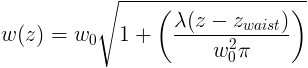
where w0 is the beam width at its minimum value, or "beam
waist," zwaist is the distance of the beam waist from the
face of the laser, and λ is the wavelength of the laser. A positive
zwaist means the waist is in front of the laser's front
face.
Our results are shown in Figure 5.
We found that the waist position was 3.6 cm behind the
front face of the laser, which must therefore be where the
surface of the output coupler mirror is. We also found
w0 = 299.3 microns, which corresponds
to a Rayleigh range [1] of 444 mm.
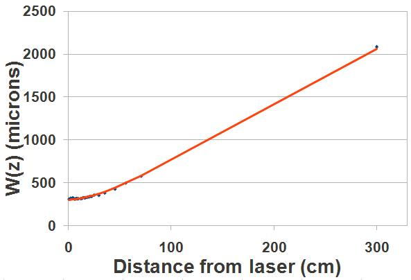
Figure 5. Measured and best-fit beam profile.
We can determine the length of the laser cavity by finding the beat frequency
between the longitudinal modes of the laser. The equation of beat frequency
is

where c is the speed of light. With help from Vince [link] we found a
beat frequency of 685.81 MHz, which corresponds to L = 21.8 cm. This result
is in reasonable agreement with our conclusion that the waist is 3.6 cm
behind the face of the laser, since the total length of the laser is 27.0 cm.
By finding the divergence of the laser beam, which explains
how the beam diffracts at large distances as the hyperbolic curve
approaches a line, we were able to calculate the wavelength of the laser
beam. The beam's divergence, theta, is described by the equation:
 [4] [4]
Equation[4] can be used to find the wavelength of
the laser beam by using the approximate slope of the curve as the
divergence. Using a divergence of 6.568 radians, and a waist size of 299.3
micrometers, we found that the wavelength of the laser was 617.58
nanometers. The error in this calculation is only 2.28 percent, when
compared to the theoretical value of the laser, which was 632
nanometers.
Conclusion
In this project we learned not only about the changing profile and propagation of
a laser beam, we also discovered how to determine the length and mirror
configuration of the laser cavity. Finally, we learned that careful measurements
of the beam profile such as ours can even be used to roughly determine the
wavelength of the laser!
References
[1] Enrique J. Galvez. "Gaussian beams in the optics course." Am. J. Phys.
74, xxx-xxx (2006).
|