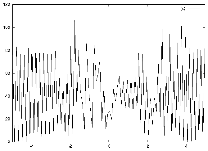
Results of Talbot effect simulations generated with gnuplot.

Thanks to Daniel Malacara for providing the expression used,
and to Maanit Desai for essential help setting this up in gnuplot. 


There are twelve .ps plots, and 12 corresponding .gifs.

There are three parameters in the calculation: N = number of slits;
d = spacing of the slits; sigma = distance to screen in units of 
the Rayleigh length. I kept d constant at 2.0 for all plots. If you
change d the plot just expands or constracts accordingly.

For the first four plots I kept sigma = 1.0 and varied N, to show
how the sharpness of the image depends on how many slits are involved.

plot 1 has N=21 (the maximum practical number in gnuplot)
plot 2 has N=3
plot 3     N=5
plot 4     N=11

Then for plots 5 through 12 I kept N=21 and varied sigma, as follows:

plot 5  sigma = 0.5
plot 6  sigma = 1.5
plot 7  sigma = 1.25
plot 8  sigma = 1.01
plot 9  sigma = 1.02
plot 10 sigma = 1.03
plot 11 sigma = 1.04
plot 12 sigma = 1.05

These plots show:

a:  the images at Sigma = .5, 1.0, 1.5
b:  the change from sharp peaks as you move away from sigma = 1.0
c:  the inversion of the pattern at sigma = 1.25 (fractional TE)

To run the program on gnuplot, start gnuplot and type:  load "talbot.txt"

To view the gnuplot code, click here.